Overview of the Election Forensics Toolkit
Test using 2024 Election Data from Georgia
Test using 2024 Election Data from Michigan
Test using 2024 Election Data from Pennsylvania
Test using 2024 Election Data from South Carolina
Overview of Eforensics
Running Eforensics
Papers Related to Eforensics
Overview of the Election Forensics Toolkit
An Election Forensics Toolkit and Guide can be found at https://www.iie.org/publications/dfg-um-publication/. It lists the Principal Investigators as Allen Hicken and Walter Mebane from the University of Michigan. It contains links to a Guide and Working Paper and begins with the following paragraph:
There is an acute need for methods of detecting and investigating fraud in elections, because the consequences of electoral fraud are grave for democratic stability and quality. When the electoral process is compromised by fraud, intimidation, or even violence, elections can become corrosive and destabilizing-sapping support for democratic institutions; inflaming suspicion; and stimulating demand for extra-constitutional means of pursuing political agendas, including violence. Accurate information about irregularities can help separate false accusations from evidence of electoral malfeasance. Accurate information about the scope of irregularities can also provide a better gauge of election quality. Finally, accurate information about the geographic location of malfeasance-the locations where irregularities occurred and how they cluster-can allow election monitors and pro-democracy organizations to focus attention and resources more efficiently and to substantiate their assessments of electoral quality.
The Guide contains the following table of Distribution and Digit Tests on page 9:
Table 1: Distribution and Digit Tests
                                                                            Value Expected in the
                                                                            Absence of Fraud or
Test                Name    Definition                                      Strategic Behavior
------------------  ------  ----------------------------------------------  ------------------
second-digit        2BL     to be compared to the mean value Benford's Law  4.187
mean                        specifies

last-digit mean     LastC   to be compared to the mean value implied by     4.5
                            uniformly distributed last digits
count
last-digit 0/5      C05s    to be compared to the mean value implied by     0.2
indicator mean              uniformly distributed last digits

percentage
last-digit 0/5      P05s    to be compared to the mean value implied by     0.2
indicator mean              uniformly distributed percentages

skewness            Skew    the extent to which a variable departs from a   0
                            normal distribution by being asymmetric

kurtosis            Kurt    the extent to which a variable departs from a   3
                            normal distribution by being spread out too
                            much or not enough

Unimodality test    DipT    tests whether the distribution of a variable    > 0.05
p-value                     departs from unimodality
There appears to be an online version of the toolkit at this link which mentions Hicken and Mebane and versions of code that mention Mebane at this link and this link. This latter link refers to a "web application sponsored by the USAID and developed by Walter Mebane and Kirill Kalinin" and the code there was used for the following test on precinct data from the 2024 U.S. general election that took place on November 5, 2024.
Test using 2024 Election Data from Georgia (20 counties with the highest populations)
Precinct data was obtained for the 20 most populous Georgia counties (according to this link) from Election Night Reporting data. It was downloaded on December 4, 2024 at 8:17 AM PST via the Media Export link at the bottom of this page of Official Results. That data was then transformed into the proper format for the Election Toolkit via the following R code:
library(tidyverse)

dd <- read_csv("precinct/ga/ga_2024_GE241204_local_precinct.csv")
names(dd) <- c("county","precinct","candidate","votes","voteType","party","office")

ee <- dd[!(dd$precinct %in% c("ALL")),]
ee$party <- toupper(ee$party)
ee <- ee[ee$party %in% c("DEM","REP"),]
ee$district <- ""

ff <- data.frame(ee$county,ee$precinct,ee$office,ee$district,ee$party,ee$candidate,ee$votes)
names(ff) <- c("county","precinct","office","district","party","candidate","votes")
write_csv(ff,"precinct/ga/20241206__ga__GE24__precinct.csv")
ff <- ff[ff$office == "President of the US",]
write_csv(ff,"precinct/ga/20241206__ga__GE24pres__precinct.csv")
ff <- ff[,c(1,2,3,5,7)]
ff <- ff %>% spread(party,votes)
ff$TOTAL <- ff$DEM + ff$REP
write_csv(ff,"precinct/ga/20241204__ga__GE24wide__precinct.csv")
The resulting file was then processed using code from this link. That code is not available as a package and was simply sourced via the following code:
library(tidyverse)
library(boot)
library(hwriter)
library(knitr)
library(kableExtra)
library(xtable)
library(moments)
library(diptest)

source("R/BasicElectionForensics.R")
source("R/BuildMap.R")
source("R/ClusterAnalysis.R")
source("R/ColorSignificance.R")
source("R/ComputeFiniteMixtureModel.R")
source("R/ComputeKlimekModel.R")
source("R/ComputeShpilkinMethod.R")


dat<-read_csv("precinct/ga/20241204__ga__GE24wide__precinct.csv")
dat <- dat[dat$TOTAL >= 10,]
tt <- table(dat$county)
tt <- tt[tt >= 20]
dat <- dat[dat$county %in% names(tt),]

#NB! R=100 to speed up computations for this example.
eldata<-BasicElectionForensics(dat,
                               Candidates=c("DEM", "REP"),
                               TotalReg ="TOTAL",
                               TotalVotes="TOTAL",
                               Level="county",
                               Methods=c("_2BL", "LastC", "C05s", "P05s",
                                         "Skew", "Kurt"))
eldata_out <- eldata$html
eldata_out <- gsub("<","<",eldata_out)
eldata_out <- gsub(">",">",eldata_out)
write(eldata_out,file="precinct/ga/eftoolkit_ga10p20_24.htm")
Following is the output of the resultant file (located online at this link):
| Level | Candidate's Name | _2BL | LastC | P05s | C05s | Skew | Kurt | Obs |
| Bibb | DEM | 3.387 | 5.548 | 0.29 | 0.161 | -0.116 | 1.451 | 31 |
| (2.387, 4.355) | (4.645, 6.484) | (0.129, 0.451) | (0.032, 0.29) | (-0.708, 0.522) | (0.732, 1.636) | |||
| Carroll | DEM | 4.536 | 4.786 | 0.107 | 0.179 | 0.583 | 2.544 | 28 |
| (3.394, 5.643) | (3.714, 6) | (-0.036, 0.214) | (0.036, 0.321) | (-0.035, 1.23) | (0.962, 3.465) | |||
| Chatham | DEM | 4.126 | 4.345 | 0.195 | 0.23 | -0.012 | 1.783 | 87 |
| (3.598, 4.666) | (3.759, 4.885) | (0.115, 0.276) | (0.138, 0.31) | (-0.293, 0.306) | (1.448, 1.991) | |||
| Cherokee | DEM | 3.452 | 4 | 0.214 | 0.238 | -0.433 | 2.752 | 42 |
| (2.619, 4.285) | (3.19, 4.81) | (0.095, 0.333) | (0.095, 0.357) | (-1.031, 0.014) | (1.726, 3.51) | |||
| Clarke | DEM | 3.917 | 4.458 | 0.167 | 0.25 | 0.77 | 3.328 | 24 |
| (2.917, 4.833) | (3.583, 5.332) | (0, 0.292) | (0.083, 0.417) | (0.252, 1.77) | (1.437, 4.779) | |||
| Clayton | DEM | 4.1 | 4.329 | 0.271 | 0.186 | -1.459 | 4.993 | 70 |
| (3.457, 4.743) | (3.615, 5) | (0.157, 0.371) | (0.1, 0.271) | (-1.99, -0.977) | (2.332, 6.717) | |||
| Cobb | DEM | 4.007 | 4.892 | 0.216 | 0.155 | 0.333 | 2.271 | 148 |
| (3.527, 4.479) | (4.426, 5.392) | (0.149, 0.284) | (0.095, 0.209) | (0.064, 0.589) | (1.848, 2.6) | |||
| Columbia | DEM | 3.978 | 4.87 | 0.174 | 0.152 | 0.479 | 3.761 | 46 |
| (3.087, 4.847) | (4.043, 5.717) | (0.065, 0.283) | (0.043, 0.239) | (-0.214, 1.279) | (2.056, 4.908) | |||
| Coweta | DEM | 4.625 | 4.208 | 0.042 | 0.125 | 1.089 | 3.192 | 24 |
| (3.333, 5.792) | (2.958, 5.416) | (-0.042, 0.083) | (-0.041, 0.25) | (0.31, 1.781) | (-0.369, 4.674) | |||
| DeKalb | DEM | 3.817 | 4.974 | 0.147 | 0.136 | -0.922 | 2.723 | 191 |
| (3.398, 4.204) | (4.581, 5.382) | (0.094, 0.199) | (0.084, 0.183) | (-1.191, -0.649) | (1.986, 3.267) | |||
| Dougherty | DEM | 3.96 | 4.44 | 0.16 | 0.16 | -0.344 | 1.597 | 25 |
| (2.88, 5) | (3.24, 5.599) | (0, 0.28) | (0, 0.28) | (-0.963, 0.421) | (0.485, 1.915) | |||
| Douglas | DEM | 3.72 | 5.6 | 0.16 | 0.08 | -0.465 | 2.547 | 25 |
| (2.72, 4.68) | (4.56, 6.72) | (0, 0.28) | (-0.04, 0.16) | (-1.192, 0.1) | (1.46, 3.489) | |||
| Effingham | DEM | 4.25 | 4.7 | 0.15 | 0.2 | 0.205 | 2.147 | 20 |
| (3.2, 5.35) | (3.451, 5.95) | (0, 0.3) | (0, 0.35) | (-0.44, 0.933) | (1.09, 2.738) | |||
| Fayette | DEM | 3.111 | 4.222 | 0.222 | 0.194 | 0.328 | 2.348 | 36 |
| (2.278, 3.889) | (3.333, 5.167) | (0.083, 0.333) | (0.028, 0.306) | (-0.274, 0.915) | (1.364, 3.099) | |||
| Forsyth | DEM | 3.966 | 4.103 | 0.276 | 0.138 | 0.018 | 2.101 | 29 |
| (3.103, 4.862) | (3.207, 4.897) | (0.103, 0.414) | (0, 0.241) | (-0.561, 0.647) | (1.249, 2.654) | |||
| Fulton | DEM | 3.952 | 4.694 | 0.218 | 0.214 | -0.696 | 2.059 | 444 |
| (3.704, 4.221) | (4.432, 4.953) | (0.18, 0.259) | (0.173, 0.25) | (-0.881, -0.499) | (1.712, 2.326) | |||
| Gwinnett | DEM | 3.615 | 4.468 | 0.167 | 0.205 | 0.06 | 2.362 | 156 |
| (3.173, 4.045) | (3.994, 4.942) | (0.109, 0.218) | (0.135, 0.269) | (-0.185, 0.279) | (2.007, 2.613) | |||
| Hall | DEM | 3.742 | 4.742 | 0.194 | 0.194 | 1.464 | 6.466 | 31 |
| (2.677, 4.871) | (3.969, 5.548) | (0.065, 0.323) | (0.065, 0.323) | (0.741, 3.032) | (3.011, 11.037) | |||
| Henry | DEM | 4.946 | 4.676 | 0.297 | 0.135 | -0.607 | 2.808 | 37 |
| (4.081, 5.865) | (3.676, 5.649) | (0.136, 0.459) | (0.027, 0.243) | (-1.222, -0.077) | (1.393, 3.743) | |||
| Muscogee | DEM | 3.72 | 4.12 | 0.2 | 0.16 | 0.205 | 1.523 | 25 |
| (2.48, 4.759) | (3, 5.2) | (0.04, 0.36) | (0.04, 0.28) | (-0.538, 0.853) | (0.386, 1.771) | |||
| Paulding | DEM | 3.905 | 4.381 | 0.095 | 0.048 | 0.565 | 3.197 | 21 |
| (2.952, 4.857) | (3, 5.619) | (-0.048, 0.19) | (-0.048, 0.095) | (-0.086, 1.636) | (1.538, 4.784) | |||
| Richmond | DEM | 4.118 | 4.368 | 0.162 | 0.25 | -0.4 | 2.105 | 68 |
| (3.5, 4.721) | (3.662, 5.074) | (0.074, 0.25) | (0.147, 0.353) | (-0.791, -0.028) | (1.368, 2.573) | |||
| Thomas | DEM | 4.1 | 4.85 | 0.3 | 0.25 | 1.41 | 3.833 | 20 |
| (2.65, 5.3) | (3.351, 6.25) | (0.1, 0.5) | (0.05, 0.4) | (0.358, 2.414) | (-1.66, 6.131) | |||
| Whitfield | DEM | 5.391 | 4.043 | 0.13 | 0.261 | 0.977 | 3.184 | 23 |
| (4.13, 6.739) | (2.87, 5.304) | (0, 0.261) | (0.087, 0.435) | (0.35, 1.821) | (0.549, 4.602) | |||
| Bibb | REP | 4.097 | 3.806 | 0.29 | 0.129 | 0.116 | 1.451 | 31 |
| (3.258, 4.871) | (3, 4.645) | (0.129, 0.419) | (0, 0.226) | (-0.524, 0.73) | (0.77, 1.635) | |||
| Carroll | REP | 4.357 | 5.571 | 0.107 | 0.214 | -0.583 | 2.544 | 28 |
| (3.321, 5.393) | (4.537, 6.5) | (0, 0.214) | (0.071, 0.357) | (-1.225, 0.039) | (1.111, 3.462) | |||
| Chatham | REP | 3.701 | 4.667 | 0.195 | 0.149 | 0.012 | 1.783 | 87 |
| (3.115, 4.241) | (4.092, 5.264) | (0.115, 0.276) | (0.069, 0.218) | (-0.278, 0.297) | (1.444, 1.99) | |||
| Cherokee | REP | 5.095 | 4.571 | 0.214 | 0.262 | 0.433 | 2.752 | 42 |
| (4.238, 6) | (3.81, 5.381) | (0.095, 0.333) | (0.119, 0.381) | (-0.014, 1.019) | (1.703, 3.464) | |||
| Clarke | REP | 3.542 | 5.375 | 0.167 | 0.167 | -0.77 | 3.328 | 24 |
| (2.251, 4.667) | (4.333, 6.375) | (0, 0.292) | (0, 0.292) | (-1.782, -0.183) | (1.139, 4.777) | |||
| Clayton | REP | 4.471 | 4.1 | 0.271 | 0.214 | 1.459 | 4.993 | 70 |
| (3.786, 5.143) | (3.4, 4.7) | (0.157, 0.371) | (0.114, 0.314) | (0.999, 1.946) | (2.492, 6.767) | |||
| Cobb | REP | 3.48 | 4.182 | 0.216 | 0.203 | -0.333 | 2.271 | 148 |
| (3.061, 3.851) | (3.676, 4.655) | (0.142, 0.277) | (0.135, 0.264) | (-0.594, -0.039) | (1.792, 2.586) | |||
| Columbia | REP | 4.435 | 4.065 | 0.174 | 0.217 | -0.479 | 3.761 | 46 |
| (3.565, 5.217) | (3.174, 4.913) | (0.065, 0.283) | (0.109, 0.326) | (-1.145, 0.186) | (2.257, 4.901) | |||
| Coweta | REP | 3.875 | 4.333 | 0.042 | 0.25 | -1.089 | 3.192 | 24 |
| (2.667, 5.124) | (3.042, 5.625) | (-0.042, 0.083) | (0.083, 0.417) | (-1.794, -0.365) | (0.092, 4.691) | |||
| DeKalb | REP | 4.403 | 4.618 | 0.147 | 0.173 | 0.922 | 2.723 | 191 |
| (3.953, 4.864) | (4.225, 5) | (0.094, 0.194) | (0.12, 0.225) | (0.649, 1.192) | (1.919, 3.269) | |||
| Dougherty | REP | 4 | 4.16 | 0.16 | 0.16 | 0.344 | 1.597 | 25 |
| (2.92, 4.92) | (3, 5.16) | (0, 0.28) | (0, 0.28) | (-0.391, 1.037) | (0.546, 1.921) | |||
| Douglas | REP | 4.04 | 4.64 | 0.16 | 0.04 | 0.465 | 2.547 | 25 |
| (2.88, 5.16) | (3.68, 5.6) | (0, 0.28) | (-0.04, 0.08) | (-0.063, 1.232) | (1.467, 3.511) | |||
| Effingham | REP | 3.65 | 5.65 | 0.15 | 0.15 | -0.205 | 2.147 | 20 |
| (2.55, 4.7) | (4.55, 6.85) | (0, 0.3) | (0, 0.3) | (-0.889, 0.419) | (0.964, 2.77) | |||
| Fayette | REP | 3.722 | 4.361 | 0.222 | 0.222 | -0.328 | 2.348 | 36 |
| (2.667, 4.639) | (3.389, 5.333) | (0.083, 0.361) | (0.083, 0.36) | (-0.968, 0.266) | (1.325, 3.091) | |||
| Forsyth | REP | 4.414 | 4.172 | 0.276 | 0.207 | -0.018 | 2.101 | 29 |
| (3.414, 5.483) | (3.345, 5.034) | (0.103, 0.448) | (0.069, 0.345) | (-0.619, 0.525) | (1.247, 2.633) | |||
| Fulton | REP | 4.022 | 4.448 | 0.218 | 0.191 | 0.696 | 2.059 | 444 |
| (3.762, 4.303) | (4.183, 4.703) | (0.18, 0.257) | (0.153, 0.225) | (0.523, 0.88) | (1.749, 2.332) | |||
| Gwinnett | REP | 4.032 | 4.109 | 0.167 | 0.218 | -0.06 | 2.362 | 156 |
| (3.603, 4.512) | (3.667, 4.564) | (0.103, 0.224) | (0.147, 0.282) | (-0.297, 0.182) | (2.005, 2.659) | |||
| Hall | REP | 4.613 | 4.871 | 0.194 | 0.194 | -1.464 | 6.466 | 31 |
| (3.614, 5.548) | (3.873, 5.87) | (0.065, 0.323) | (0.065, 0.323) | (-3.055, -0.78) | (3.387, 10.992) | |||
| Henry | REP | 3.757 | 4.108 | 0.297 | 0.189 | 0.607 | 2.808 | 37 |
| (2.919, 4.595) | (3.162, 5.027) | (0.135, 0.432) | (0.054, 0.297) | (0.091, 1.195) | (1.517, 3.804) | |||
| Muscogee | REP | 4.52 | 5.04 | 0.2 | 0.28 | -0.205 | 1.523 | 25 |
| (3.201, 5.76) | (4.04, 6.079) | (0.04, 0.359) | (0.08, 0.44) | (-0.868, 0.506) | (0.492, 1.776) | |||
| Paulding | REP | 3.762 | 4.238 | 0.095 | 0.048 | -0.565 | 3.197 | 21 |
| (2.81, 4.808) | (3.239, 5.381) | (-0.048, 0.19) | (-0.048, 0.095) | (-1.629, 0.198) | (1.109, 4.797) | |||
| Richmond | REP | 3.897 | 4.294 | 0.162 | 0.235 | 0.4 | 2.105 | 68 |
| (3.177, 4.529) | (3.515, 5.059) | (0.059, 0.25) | (0.132, 0.338) | (-0.024, 0.817) | (1.323, 2.602) | |||
| Thomas | REP | 4.45 | 5.5 | 0.3 | 0.15 | -1.41 | 3.833 | 20 |
| (3.151, 5.7) | (4.251, 6.8) | (0.1, 0.5) | (-0.05, 0.3) | (-2.324, -0.346) | (-1.961, 5.995) | |||
| Whitfield | REP | 3.783 | 4.565 | 0.13 | 0.304 | -0.977 | 3.184 | 23 |
| (2.61, 4.999) |
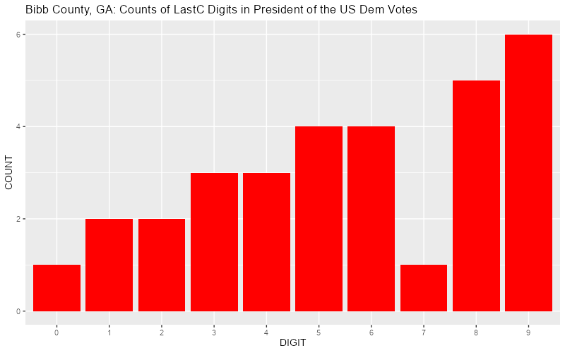
The output appears to consist of pairs of rows with the first pair containing the specified value and the seoond line containing the 95 percent confidence limits). The specified values appear to be red if the 95 percent confidence limits do not include the expected value. For example, the LastC value of 5.548 for DEM for Bibb County is colored red because its 95% confidence limits of 4.645 and 6.484 do not include the expected value of 4.5. LastC is the last digit of the value being measured (in this case, Democrat vote count) and, if it were to contain random digits between 0 and 9, the average would be expected to be 4.5. The histogram below shows the actual distribution of the digits:

As can be seen, there are noticably more occurrances of the digits 8 and 9 than any of the other digits. Also, except for the digit 7, the counts of the digits generally increase from left to right. It should be noted that these counts exclude any precincts with fewer that 10 votes, chiefly to avoid precincts with no votes increasing the count of digit 0. However, this raises the question of what are the best next steps to take to determine if a red flag is actually a problem.
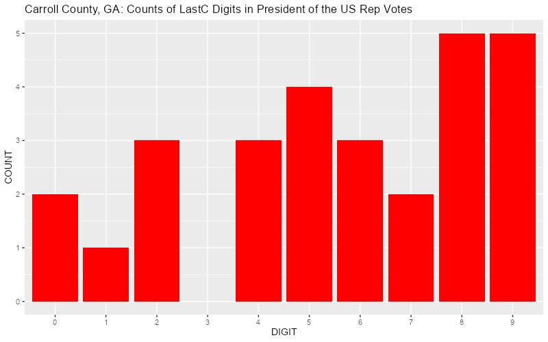
Regarding the LastC test, following are two other vote counts that had red flags:
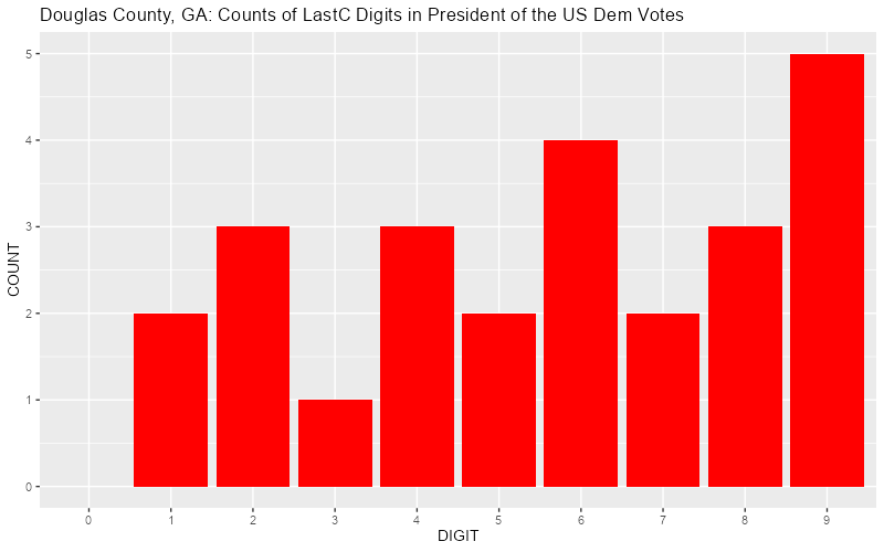
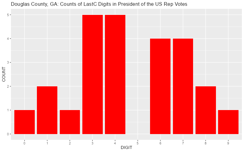
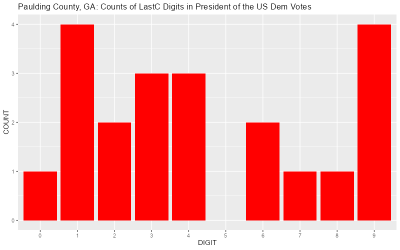
Note that, like Bibb County, the counts of the digits generally increase from left to right. Even more interesting distributions can be seen in those vote counts that had red flags for the C05s test:
As can be seen, the distribution counta for the Democrat and Republican votes in both Douglas and Paulding counties is zero for either the 0 or the 5 digit. For the other digit, the distribution count is one except for the Democrat votes in Douglas County for which it is 2. Also interesting is that the expected value of 0.2 falls far outside the confidence limits for all 4 tests. Those 4 tests had upper confidence limits of 0.16, 0.095, 0.08, and 0.095, far less than the expected value of 0.2. Finally, the two counties border each other, just northwest of Fulton County. There are of course differing reasons, some likely bnign, why this may have occurred. But, if there was any human manipulation involved, it could be that the "round digits" of 0 and 5 were unintentially avoided.
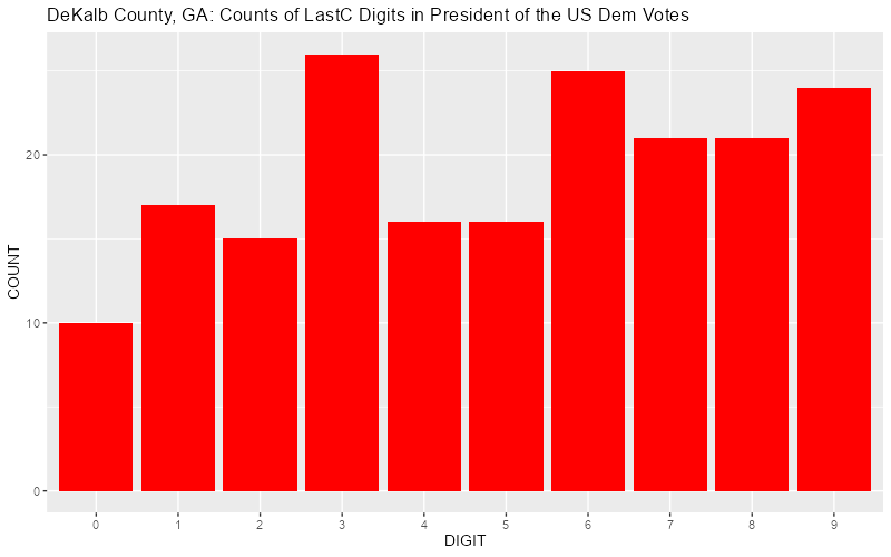
The other vote count that failed the C05s test was the Democrat vote count in DeKalb County. As seem in its distribution shown earlier, the counts for the 0 and 5 digits were lower in DeKalb County, same as the prior 4 tests.

Test using 2024 Election Data from Michigan
| Level | Candidate's Name | _2BL | LastC | P05s | C05s | Skew | Kurt | Obs |
| MIEaton | Turnout | 4.455 | 4.295 | 0.295 | 0.25 | -0.535 | 3.064 | 44 |
| (3.682, 5.34) | (3.432, 5.114) | (0.159, 0.432) | (0.114, 0.364) | (-1.209, -0.093) | (1.913, 3.962) | |||
| MIGrand_Traverse | Turnout | 3.949 | 4.128 | 0.128 | 0.205 | -0.613 | 2.923 | 39 |
| (3.206, 4.744) | (3.256, 5.026) | (0.026, 0.205) | (0.077, 0.333) | (-1.205, -0.128) | (1.636, 3.899) | |||
| MIMacomb | Turnout | 4.097 | 4.578 | 0.172 | 0.188 | -0.758 | 3.755 | 308 |
| (3.792, 4.399) | (4.244, 4.909) | (0.13, 0.214) | (0.146, 0.231) | (-1.113, -0.464) | (2.991, 4.649) | |||
| MIOakland | Turnout | 3.988 | 4.558 | 0.187 | 0.191 | -1.599 | 6.38 | 498 |
| (3.743, 4.227) | (4.305, 4.817) | (0.149, 0.219) | (0.157, 0.225) | (-1.894, -1.335) | (5.054, 7.698) | |||
| MIEaton | DEM | 3.932 | 4.909 | 0.227 | 0.091 | 0.229 | 2.172 | 44 |
| (3.114, 4.75) | (4.068, 5.727) | (0.091, 0.341) | (0, 0.159) | (-0.238, 0.832) | (1.364, 2.811) | |||
| MIGrand_Traverse | DEM | 2.846 | 4.846 | 0.154 | 0.128 | 0.147 | 2.503 | 39 |
| (1.924, 3.744) | (3.872, 5.769) | (0.026, 0.256) | (0, 0.231) | (-0.292, 0.654) | (1.588, 3.089) | |||
| MIMacomb | DEM | 4.023 | 4.601 | 0.214 | 0.205 | 0.993 | 4.089 | 308 |
| (3.679, 4.357) | (4.282, 4.916) | (0.169, 0.256) | (0.156, 0.25) | (0.757, 1.252) | (3.264, 4.874) | |||
| MIOakland | DEM | 3.662 | 4.275 | 0.195 | 0.217 | 0.749 | 2.831 | 498 |
| (3.38, 3.912) | (4.014, 4.512) | (0.159, 0.229) | (0.183, 0.251) | (0.625, 0.889) | (2.468, 3.179) | |||
| MIEaton | REP | 4.045 | 4.136 | 0.159 | 0.227 | -0.192 | 2.128 | 44 |
| (3.136, 4.931) | (3.318, 4.977) | (0.045, 0.25) | (0.091, 0.341) | (-0.775, 0.289) | (1.448, 2.712) | |||
| MIGrand_Traverse | REP | 3.821 | 4.436 | 0.179 | 0.103 | -0.08 | 2.468 | 39 |
| (2.949, 4.692) | (3.564, 5.308) | (0.051, 0.282) | (0, 0.179) | (-0.542, 0.385) | (1.573, 3.062) | |||
| MIMacomb | REP | 4.062 | 4.513 | 0.208 | 0.221 | -0.875 | 3.762 | 308 |
| (3.74, 4.396) | (4.182, 4.831) | (0.159, 0.25) | (0.179, 0.266) | (-1.108, -0.651) | (3.042, 4.41) | |||
| MIOakland | REP | 3.716 | 4.42 | 0.211 | 0.215 | -0.664 | 2.727 | 498 |
| (3.473, 3.979) | (4.177, 4.665) | (0.177, 0.245) | (0.177, 0.249) | (-0.79, -0.537) | (2 |
Test using 2024 Election Data from Pennsylvania
Precinct voting results and registration data was obtained for all Pennsylvania counties at the following URLs:
Bulk Election Data for Pennsylvania:
That data was then transformed into the proper format for the Election Toolkit and used to generate the following output:
| x | |||||||||||||||||||||||||||||||||||||||||||||||||||||||||||||||||||||||||||||||||||||||||||||||||||||||||||||||||||||||||||||||||||||||||||||||||||||||||||||||||||||||||||||||||||||||||||||||||||||||||||||||||||||||||||||||||||||||||||||||||||||||||||||||||||||||||||||||||||||||||||||||||||||||||||||||||||||||||||||||||||||||||||||||||||||||||||||||||||||||||||||||||||||||||||||||||||||||||||||||||||||||||||||||||||||||||||||||||||||||||||||||||||||||||||||||||||||||||||||||||||||||||||||||||||||||||||||||||||||||||||||||||||||||||||||||||||||||||||||||||||||||||||||||||||||||||||||||||||||||||||||||||||||||||||||||||||||||||||||||||||||||||||||||||||||||||||||||||||||||||||||||||||||||||||||||||||||||||||||||||||||||||||||||||||||||||||||||||||||||||||||||||||||||||||||||||||||||||||||||||||||||||||||||||||||||||||||||||||||||||||||||||||||||||||||||||||||||||||||||||||||||||||||||||||||||||||||||||||||||||||||||||||||||||||||||||||||||||||||||||||||||||||||||||||||||||||||||||||||||
|---|---|---|---|---|---|---|---|---|---|---|---|---|---|---|---|---|---|---|---|---|---|---|---|---|---|---|---|---|---|---|---|---|---|---|---|---|---|---|---|---|---|---|---|---|---|---|---|---|---|---|---|---|---|---|---|---|---|---|---|---|---|---|---|---|---|---|---|---|---|---|---|---|---|---|---|---|---|---|---|---|---|---|---|---|---|---|---|---|---|---|---|---|---|---|---|---|---|---|---|---|---|---|---|---|---|---|---|---|---|---|---|---|---|---|---|---|---|---|---|---|---|---|---|---|---|---|---|---|---|---|---|---|---|---|---|---|---|---|---|---|---|---|---|---|---|---|---|---|---|---|---|---|---|---|---|---|---|---|---|---|---|---|---|---|---|---|---|---|---|---|---|---|---|---|---|---|---|---|---|---|---|---|---|---|---|---|---|---|---|---|---|---|---|---|---|---|---|---|---|---|---|---|---|---|---|---|---|---|---|---|---|---|---|---|---|---|---|---|---|---|---|---|---|---|---|---|---|---|---|---|---|---|---|---|---|---|---|---|---|---|---|---|---|---|---|---|---|---|---|---|---|---|---|---|---|---|---|---|---|---|---|---|---|---|---|---|---|---|---|---|---|---|---|---|---|---|---|---|---|---|---|---|---|---|---|---|---|---|---|---|---|---|---|---|---|---|---|---|---|---|---|---|---|---|---|---|---|---|---|---|---|---|---|---|---|---|---|---|---|---|---|---|---|---|---|---|---|---|---|---|---|---|---|---|---|---|---|---|---|---|---|---|---|---|---|---|---|---|---|---|---|---|---|---|---|---|---|---|---|---|---|---|---|---|---|---|---|---|---|---|---|---|---|---|---|---|---|---|---|---|---|---|---|---|---|---|---|---|---|---|---|---|---|---|---|---|---|---|---|---|---|---|---|---|---|---|---|---|---|---|---|---|---|---|---|---|---|---|---|---|---|---|---|---|---|---|---|---|---|---|---|---|---|---|---|---|---|---|---|---|---|---|---|---|---|---|---|---|---|---|---|---|---|---|---|---|---|---|---|---|---|---|---|---|---|---|---|---|---|---|---|---|---|---|---|---|---|---|---|---|---|---|---|---|---|---|---|---|---|---|---|---|---|---|---|---|---|---|---|---|---|---|---|---|---|---|---|---|---|---|---|---|---|---|---|---|---|---|---|---|---|---|---|---|---|---|---|---|---|---|---|---|---|---|---|---|---|---|---|---|---|---|---|---|---|---|---|---|---|---|---|---|---|---|---|---|---|---|---|---|---|---|---|---|---|---|---|---|---|---|---|---|---|---|---|---|---|---|---|---|---|---|---|---|---|---|---|---|---|---|---|---|---|---|---|---|---|---|---|---|---|---|---|---|---|---|---|---|---|---|---|---|---|---|---|---|---|---|---|---|---|---|---|---|---|---|---|---|---|---|---|---|---|---|---|---|---|---|---|---|---|---|---|---|---|---|---|---|---|---|---|---|---|---|---|---|---|---|---|---|---|---|---|---|---|---|---|---|---|---|---|---|---|---|---|---|---|---|---|---|---|---|---|---|---|---|---|---|---|---|---|---|---|---|---|---|---|---|---|---|---|---|---|---|---|---|---|---|---|---|---|---|---|---|---|---|---|---|---|---|---|---|---|---|---|---|---|---|---|---|---|---|---|---|---|---|---|---|---|---|---|---|---|---|---|---|---|---|---|---|---|---|---|---|---|---|---|---|---|---|---|---|---|---|---|---|---|---|---|---|---|---|---|---|---|---|---|---|---|---|---|---|---|---|---|---|---|---|---|---|---|---|---|---|---|---|---|---|---|---|---|---|---|---|---|---|---|---|---|---|---|---|---|---|---|---|---|---|---|---|---|---|---|---|---|---|---|---|---|---|---|---|---|---|---|---|---|---|---|---|---|---|---|---|---|---|---|---|---|---|---|---|---|---|---|---|---|---|---|---|---|---|---|---|---|---|---|---|---|---|---|---|---|---|---|---|---|---|---|---|---|---|---|---|---|---|---|---|---|---|---|---|---|---|---|---|---|---|---|---|---|---|---|---|---|---|---|---|---|---|---|---|---|---|---|---|---|---|---|---|---|---|---|---|---|---|---|---|---|---|---|---|---|---|---|---|---|---|---|---|---|---|---|---|---|---|---|---|---|---|---|---|---|---|---|---|---|---|---|---|---|---|---|---|---|---|---|---|---|---|---|---|---|---|---|---|---|---|---|---|---|---|---|---|---|---|---|---|---|---|---|---|---|---|---|---|---|---|---|
For Cameron County, the value of 5.8 is red flagged for the Candidate's Name of DEM and indicator LastC (fourth column). In the same column of the row below the 5.8 is the interval "(4.7, 7)". This is the 95 percent confidence interval. The reason that this item is red flagged is that LastC is the average of the last digit in the precinct vote totals. Since this last digit can vary from 0 to 9, the expected average is 4.5. Because 4.5 lies outside the confidence interval of (4.7, 7), it is therefore red flagged. Cameron County has just 10 precincts and the vote totals for the 10 precincts are 2,46,69,147,16,15,37,16,73, and 117. The last digits of these 10 numbers are 2,6,9,7,6,5,7,6,3, and 7. These add up to 58 for an average of 5.8. This is the number shown in red above. There might actually be a good argument for filtering out vote totals below 10 at least since those might tend to be smaller numbers averaging less than 4.5. In this case, this would have given a total of 9 numbers of 56 for an average of 6.2. In any case, the following plot shows the distribution of the last digit of the 10 numbers:
Following is the distribution of the last digit of the 10 numbers for the Candidate's Name of REP. The table above shows that the LastC indicator variable in this case was 4.4 with a 95% confidence interval of (2.5, 6.3). This interval does contain the expected average of 4.5 so this value is not red flagged.
The above example does show a possible weakness of this indicator. It appears to key strictly on the average. Hence, if half of the values were zero and the other half were 9, it would appear that this distribution would not be red flagged. This case of an uneven distribution might be addressed in some of the other indicators. I would seem useful to get a similar understanding of these other indicators, especially Skew and Kurt which have to do with the Skewness and Kurtosis, statistical measures that describe the shape of a distribution of data.
Precinct data was obtained for 6 South Carolina counties from Election Night Reporting data from the following 6 URLs: These files were downloaded on November 28, 2024 at 1:23 AM PST via the Detail XLS links on the above pages and the election data extracted. That data was then transformed into the proper format for the Election Toolkit via the following R code:
library(tidyverse)

counties <- c("SCAiken","CSChesterfield","SCDarlington",
              "SCLee","SCMarlboro","SCSumter")
dd <- read_csv("SClastfocus/20241127__sc__last_focus__precinct.csv")

dd$candidate[dd$office == "Registered Voters"] <- "R_V"
dd$candidate[dd$office == "Ballots Cast"] <- "B_C"
dd$office[dd$office == "Registered Voters"] <- "President and Vice President (Vote For 1)"
dd$office[dd$office == "Ballots Cast"] <- "President and Vice President (Vote For 1)"

ee <- dd[dd$office == "President and Vice President (Vote For 1)",]
ee <- ee[!(ee$precinct %in% c("Failsafe","Failsafe Provisional","Provisional","Total:")),]
ee$party <- substring(ee$candidate,1,3)
ee <- ee[ee$party %in% c("DEM","REP","R_V","B_C"),]
ff <- data.frame(ee$county,ee$precinct,ee$office,ee$party,ee$votes)
names(ff) <- c("county","precinct","office","party","votes")
ff <- ff %>% spread(party,votes)
ff$TOTAL <- ff$DEM + ff$REP
write_csv(ff,"SClastfocus/20241127__sc__last_focus__wide2.csv")
The resulting file was then processed using code from this link. That code is not available as a package and was simply sourced via the following code:
library(tidyverse)
library(boot)
library(hwriter)
library(knitr)
library(kableExtra)
library(xtable)
library(moments)
library(diptest)

source("R/BasicElectionForensics.R")
source("R/BuildMap.R")
source("R/ClusterAnalysis.R")
source("R/ColorSignificance.R")
source("R/ComputeFiniteMixtureModel.R")
source("R/ComputeKlimekModel.R")
source("R/ComputeShpilkinMethod.R")

dat<-read_csv("SClastfocus/20241127__sc__last_focus__wide2.csv")

#NB! R=100 to speed up computations for this example.
eldata<-BasicElectionForensics(dat,
                               Candidates=c("DEM", "REP"),
                               TotalReg="R_V",
                               TotalVotes="B_C",
                               Level="county",
                               Methods=c("_2BL", "LastC", "C05s", "P05s",
                                         "Skew", "Kurt"))
eldata_out <- eldata$html
eldata_out <- gsub("<","<",eldata_out)
eldata_out <- gsub(">",">",eldata_out)
write(eldata_out,file="eftoolkit_sc6_24.htm")
Following is the output of the resultant file (located online at this link):
The output appears to consist of pairs of rows with the first pair containing the specified value and the seoond line containing the 95 percent confidence limits). The specified values appear to be red if the 95 percent confidence limits do not include the expected value. For example, the LastC value of 3.764 for DEM for SCAiken (Aiken County, South Carolina) is colored red because its 95% confidence limits of 3.135 and 4.326 do not include the expected value of 4.5. LastC is the last digit of the value being measured (in this case, Democrat vote count) and, if it were to contain random digits between 0 and 9, the average would be expected to be 4.5. The histogram below shows the actual distribution of the digits:
As can be seen, there are noticably more occurrances of the digits 1 and 2 than any of the other digits. Also, there are almost double the occurances of the first three digits (0, 1, and 2) as the last three digits (7, 8, and 9). As before, this raises the question of what are the best next steps to take to determine if a red flag is actually a problem. By pure chance, one would expect about 1 out of every 20 values to be outside of the 95% confidence limits. One step might be to look at the actual distribution of the digits as was done here. It would appear that this red flag is based strictly on the average of the digits. However, it's unclear how one could best judge if the distribution of the digits adds or subtracts from the likelihood that this represents a real problem. It might also be possible to make a judgement based on the number of tests that fall outside the 95% confidence limits for a county. For example, the DEM vote count for Aiken County falls outside the limits in 3 tests (LastC, Skew, and Kurtosis). In addition, it might make sense to look at the test with smaller confidence limits though it is not clear how to do this in the current code. Of course, the final solution for anomalies in elections is to audit or recount the balance. Still, it would be preferable to do as much other analysis as possible before this. Also, it's not clear whether or not every or most precincts in the flagged county would need to be audited or recounted. These numerical tests would seem very useful in flagging potential problems but it would also seem useful to understand how best to follow up on those counties and values that are flagged. In recent years, Walter Mebane has been working on a measurement model called eforensics for measuring election frauds. A March 6, 2022 paper titled Measuring Election Frauds*" contains the following abstract: "A measurement model called eforensics produces valid estimates of the incidence and magnitude of election frauds, using as input aggregation unit counts of eligible voters and of votes for the ballot alternatives. While valid, the estimates are imperfect: eforensics cannot detect procedural defects, measures only frauds that benefit one alternative and is sensitive to things - particularly elector strategic behavior and election administration weaknesses - not produced by the kinds of malevolent distortions of elector intentions that constitute genuine frauds. eforensics parameters support distinguishing results of malevolent distortions from results of strategic behavior. We use 32 real elections to demonstrate that eforensics measures the magnitude of election frauds at aggregation units such as polling stations, precincts or ballot boxes." On January 18, 2023, Mebane was interviewed by the "Not Another Political Podcast" on eforensics. The full interview, along with a full transcript, can be found at the prior link. In addition, Mebane gave a talk titled Election Forensics: Detecting Election Fraud for the National Press Foundation. A transcript, Mebane's slides, and a YouTube video of the talk can be found at the prior link. Other papers by Mebane can be found on his University of Michigan web site. A paper from June 29, 2023 titled "Lost Votes and Posterior Multimodality in the eforensics Model" is 105 pages and goes pretty deeply into eforensics. It was prepared for presentation at PolMeth 2023, Stanford University, Palo Alto CA. His most recent paper is titled "eforensics Analysis of the 2024 President Election in Pennsylvania". Regarding the analysis, the paper states the following: "The active eforensics-frauds magnitudes shown in Figure 2 suggest it is a close call - or perhaps more precisely a highly focused call - to say whether the eforensics estimates reported in Table 3 mean the election was decided or nearly decided by malevolent distortions of electors' intentions. Regarding this conclusion, a PR Newswire article states the following: Mebane's analysis examines 7,040,360 votes across 67 Pennsylvania counties. The eforensics model estimates that between 25,000 and 225,440 votes in the Presidential race were possibly fraudulent. The range is due to Dr. Mebane applying several different forensic models in completing his evaluation. The code for eforensics appears to be located at both on GitHub and on a site of R Package Documentation. Both sites list the version as 0.0.4. The latter site seems to have a little more functionality. For example, the left margin contains a link to the man page for the eforensics command. At the end of that man page is a code example that calls that command.
|