A study titled "STEM Workers, H-1B Visas, and Productivity in US Cities", written by economist Giovanni Peri, Kevin Shih, and Chad Sparber, was released by the Journal of Labor Economics on July 1, 2015. Following is the last paragraph of the study's conclusion:
We find that a 1 percentage point increase in the foreign STEM share of a city’s total employment increased the wage growth of native college-educated labor by about 7–8 percentage points and the wage growth of non-college-educated natives by 3–4 percentage points. We find insignificant effects on the employment of those two groups. These results indicate that STEM workers spur economic growth by increasing productivity, especially that of college-educated workers.
That is almost identical to the last paragraph of the version of the paper at this link except that it omits the following final sentence:
They also experienced increasing housing rents, which eroded part of their wage gain.
In any case, the study contains the following numbers in the first row of Table 5:
Table 5: The Effects of Foreign STEM on Native Wages and Employment

                       Weekly Wage,  Weekly Wage,    Weekly Wage,        Employment,  Employment,     Employment,
Explanatory Variable:  Native STEM   Native College  Native Non-College  Native STEM  Native College  Native Non-College
Growth Rate of                       educated        educated                         educated        educated
Foreign–STEM                (1)            (2)            (3)                 (4)            (5)            (6)
---------------------  ------------  --------------  ------------------  -----------  --------------  ------------------
(a) Baseline 2SLS;         6.65           8.03***        3.78**              0.53           2.48           5.17
O*NET 4% Definition       (4.53)         (3.03)         (1.75)              (0.56)         (4.69)         (4.20)

  * Significant at the 10% level.
 ** Significant at the 5% level.
*** Significant at the 1% level.
These are almost identical to the numbers in Table 6 at the aforementioned link. One big difference is that the top number (the slope) for the last column is 5.17 in the paper but -5.17 in the link. In fact, Giovanni Peri sent me a 30 April, 2014 version of this paper in which the value was likewise -5.17. Hence, it appears that this was an error in the study, at least in the initial Journal of Labor Statistics version.
3. Replication of Six Key Findings Using Study's Data
Following are the statements that generate the 6 regressions from which the values in the first row of Table 5 are derived. They are taken from the file Table_5_April_30_2014.do:
*Table 5, row (a)
* explanatory is STEM O*net definition 4%, coefficients (1)-(6) in order
xi: ivreg2 delta_native_stemO4_wkwage (delta_imm_stemO4 = delta_imm_stemO4_H1B_hat80) bartik_coll_wage bartik_coll_emp i.year i.metarea if year>1990 & panel1980==1, robust cluster(metarea)
test delta_imm_stemO4==8.03
xi: ivreg2 delta_native_coll_wkwage (delta_imm_stemO4 = delta_imm_stemO4_H1B_hat80) bartik_coll_wage bartik_coll_emp i.year i.metarea if year>1990 & panel1980==1, robust cluster(metarea)
xi: ivreg2 delta_native_nocoll_wkwage (delta_imm_stemO4 = delta_imm_stemO4_H1B_hat80) bartik_nocoll_wage bartik_nocoll_emp i.year i.metarea if year>1990 & panel1980==1, robust cluster(metarea)
xi: ivreg2 delta_native_stemO4_emp (delta_imm_stemO4 = delta_imm_stemO4_H1B_hat80) bartik_coll_wage bartik_coll_emp i.year i.metarea if year>1990 & panel1980==1, robust cluster(metarea)
xi: ivreg2 delta_native_coll_emp (delta_imm_stemO4 = delta_imm_stemO4_H1B_hat80) bartik_coll_wage bartik_coll_emp i.year i.metarea if year>1990 & panel1980==1, robust cluster(metarea)
xi: ivreg2 delta_native_nocoll_emp (delta_imm_stemO4 = delta_imm_stemO4_H1B_hat80) bartik_nocoll_wage bartik_nocoll_emp i.year i.metarea if year>1990 & panel1980==1, robust cluster(metarea)
An attempt to replicate the six key slopes in row 1 of Table 5 was made in the R language using the ivreg function in the AER package. The following table shows the results:
[1] " N  INTERCEPT    SLOPE    STUDY    % DIFF     S.E.   T-STAT    P-VAL  DESCRIPTION"
[1] "--  ---------  --------  -------  -------  -------  -------  -------  -----------------------------------"
[1] "1990-2010 USING STUDY'S FORMULA"
[1] " 1)   -0.3322    6.6191   6.6500    -0.46    7.073    0.936    0.350  Weekly Wage, Native STEM"
[1] " 2)   -0.0764    8.0414   8.0300     0.14    3.804    2.114    0.035  Weekly Wage, Native College-Educated"
[1] " 3)    0.0594    3.6174   3.7800    -4.30    1.972    1.835    0.067  Weekly Wage, Native Non-College-Educated"
[1] " 4)    0.0272    0.5349   0.5300     0.92    0.296    1.806    0.072  Employment, Native STEM"
[1] " 5)    0.0311    2.4942   2.4800     0.57    1.452    1.718    0.087  Employment, Native College-Educated"
[1] " 6)   -0.2557   -5.1701  -5.1700     0.00    3.178   -1.627    0.104  Employment, Native Non-College-Educated"
As can be seen in the column labeled % DIFF, all 6 slopes were within one percent of the study's values except for the weekly wage for native non-college-educated workers which was within 4.3 percent of the study's value.
4. An Initial Look at the Data
Following is a list and brief description of the variables used in the six multivariate regressions above:
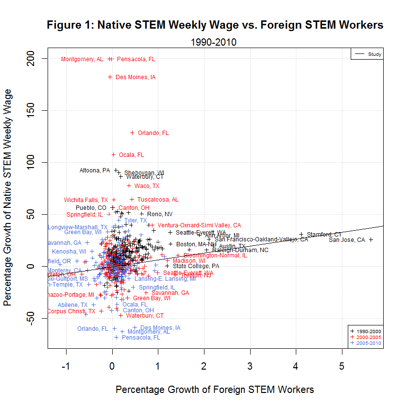
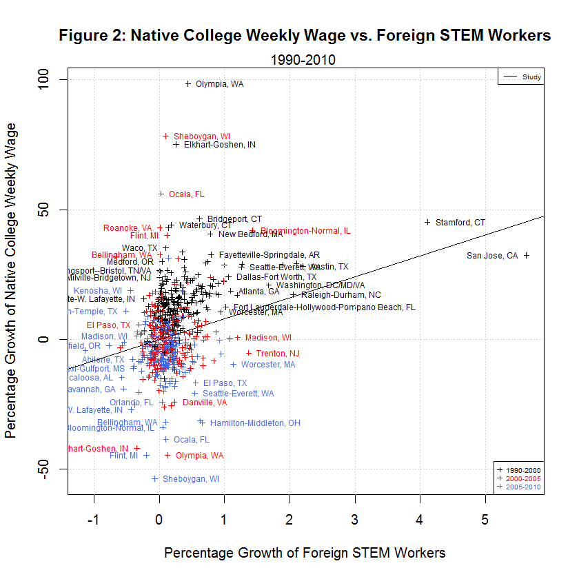
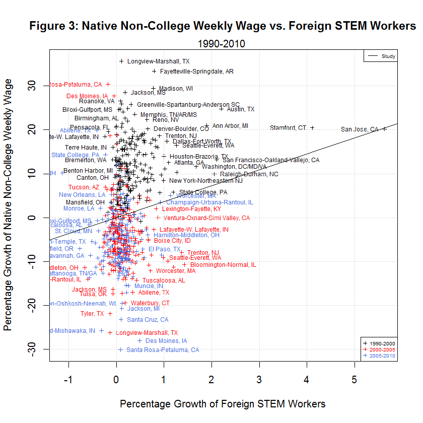
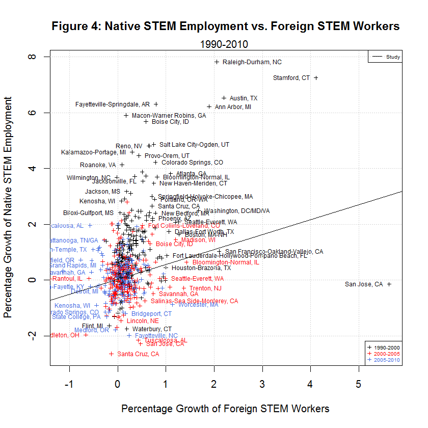
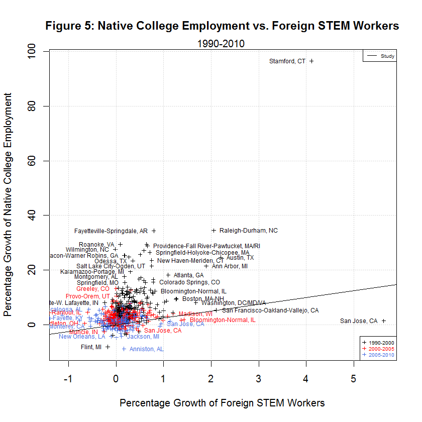
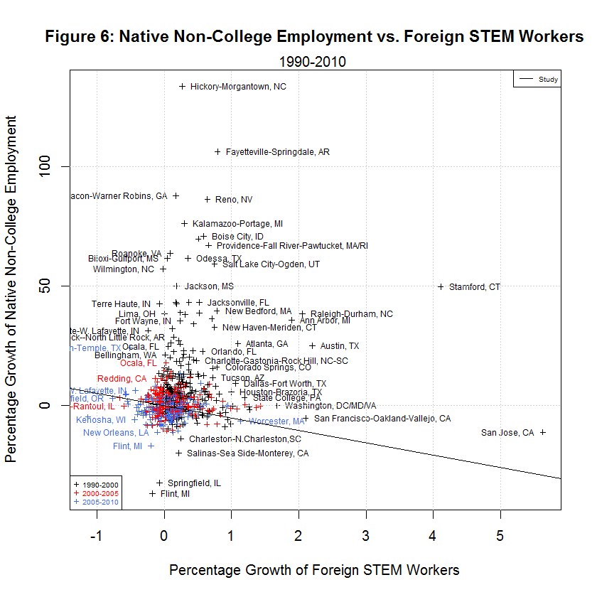
delta_native_stemO4_wkwage - key dependent variable for growth in Native STEM Weekly Wage
delta_native_coll_wkwage   - key dependent variable for growth in Native College-educated Weekly Wage
delta_native_nocoll_wkwage - key dependent variable for growth in Native Non-College-educated Weekly Wage
delta_native_stemO4_emp    - key dependent variable for growth in Native STEM Employment
delta_native_coll_emp      - key dependent variable for growth in Native College-educated Employment
delta_native_nocoll_emp    - key dependent variable for growth in Native Non-College-educated Employment
delta_imm_stemO4           - key independent variable for growth in Immigrant STEM
delta_imm_stemO4_H1B_hat80 - instrument for H-1B imputed growth of foreign STEM
bartik_coll_wage           - instrument to predict the wage growth of college-educated workers based on each city’s industrial composition in 1980
bartik_coll_emp            - instrument to predict the employment growth of college-educated workers based on each city’s industrial composition in 1980
bartik_nocoll_wage         - instrument to predict the wage growth of non-college-educated workers based on each city’s industrial composition in 1980
bartik_nocoll_emp          - instrument to predict the employment growth of non-college-educated workers based on each city’s industrial composition in 1980
i.year                     - indicator or dummy variable for the year span (1990-2000, 2000-2005, and 2005-2010)
i.metarea                  - indicator or dummy variable for the 219 metropolitan areas
Before looking at the regressions used by the study, it helps to look at the following plots of the six dependent variables versus the main regressor, the growth in immigrant STEM (delta_imm_stemO4):
One thing evident in the six plots is that the growth in the dependent variables along the y-axis was generally best from 1990 to 2000, next best from 2000-2005, and worst from 2005-2010. The following table shows the averages of the independent and six dependent variables during the three time spans:
[1] "AVERAGES OF INDEPENDENT AND SIX DEPENDENT VARIABLES IN STUDY'S ORIGINAL DATA"
[1] ""
[1] " N  1990-2000  2000-2005  2005-2010  Variable"
[1] "--  ---------  ---------  ---------  --------"
[1] " 0)    0.3827     0.1375     0.0701  Foreign STEM Workers"
[1] " 1)   15.0447     6.9259    -1.2507  Native STEM Weekly Wage"
[1] " 2)   15.3769     1.4646    -5.7251  Native College Weekly Wage"
[1] " 3)   12.2605    -3.9557    -4.9925  Native Non-College Weekly Wage"
[1] " 4)    1.3310     0.0738     0.1278  Native STEM Employment"
[1] " 5)    8.5920     2.9037     1.4123  Native College Employment"
[1] " 6)   12.3931     1.4488    -1.3758  Native Non-College Employment"
As can be seen, the average growth rates were all highest from 1990 to 2000, next highest from 2000-2005, and lowest from 2005-2010 with a single exception. That exception is Native STEM Employment for which the lowest rate was 2000-2005. That's not surprising since this includes the tech crash. In addition, the data shows negative averages for all of the growth in weekly wages and for native non-college employment from 2005 to 2010. It also shows negative average growth for native non-college weekly wages from 2000-2005. It seems that non-college workers have had an especially tough time since 2000.
5. The Use of Time Spans of Different Length
In fact, a close look at the data reveals a serious problem. As stated above, the three time spans are 1990-2000, 2000-2005, and 2005-2010. Hence, the first one is a 10-year span and the second and third are 5-year spans. As is likely the case with most readers of the study, I assumed that the different lengths were accounted for somehow, perhaps by using annualized growth figures. In fact, the figures are not annualized but are for the entire span. Following are the formulas for the dependent variables and instruments, taken from file Table_5_April_30_2014.do:
gen delta_native_stemO4_wkwage=(nat_stemO4_wkwage-nat_stemO4_wkwage[_n-1])/nat_stemO4_wkwage[_n-1] if year>=1980
gen delta_native_coll_wkwage=(nat_coll_wkwage-nat_coll_wkwage[_n-1])/nat_coll_wkwage[_n-1] if year>=1980
gen delta_native_nocoll_wkwage=(nat_nocoll_wkwage-nat_nocoll_wkwage[_n-1])/nat_nocoll_wkwage[_n-1] if year>=1980
gen delta_native_stemO4_emp=(nat_stemO4_emp-nat_stemO4_emp[_n-1])/labforce[_n-1] if year>=1980
gen delta_native_coll_emp=(nat_coll_emp-nat_coll_emp[_n-1])/labforce[_n-1] if year>=1980
gen delta_native_nocoll_emp=(nat_nocoll_emp-nat_nocoll_emp[_n-1])/labforce[_n-1] if year>=1980
gen delta_imm_stemO4=(imm_stemO4-imm_stemO4[_n-1])/labforce[_n-1] if year>=1980
gen delta_imm_stemO4_H1B_hat80=(imm_stemO4_H1B_hat80-imm_stemO4_H1B_hat80[_n-1])/labforce_hat80[_n-1] if year>=1990
gen bartik_coll_wage=(pred_coll_wkwage-pred_coll_wkwage[_n-1])/pred_coll_wkwage[_n-1] if year>1990
gen bartik_nocoll_wage=(pred_nocoll_wkwage-pred_nocoll_wkwage[_n-1])/pred_nocoll_wkwage[_n-1] if year>1990
gen bartik_coll_emp=(pred_coll_emp-pred_coll_emp[_n-1])/pred_emp[_n-1] if year>1990
gen bartik_nocoll_emp=(pred_nocoll_emp-pred_nocoll_emp[_n-1])/pred_emp[_n-1] if year>1990
Following are the same formulas with spacing added so that their similar structures and be compared:
gen delta_native_stemO4_wkwage=(nat_stemO4_wkwage   -nat_stemO4_wkwage[_n-1])   /nat_stemO4_wkwage[_n-1]  if year>=1980
gen delta_native_coll_wkwage  =(nat_coll_wkwage     -nat_coll_wkwage[_n-1])     /nat_coll_wkwage[_n-1]    if year>=1980
gen delta_native_nocoll_wkwage=(nat_nocoll_wkwage   -nat_nocoll_wkwage[_n-1])   /nat_nocoll_wkwage[_n-1]  if year>=1980
gen delta_native_stemO4_emp   =(nat_stemO4_emp      -nat_stemO4_emp[_n-1])      /labforce[_n-1]           if year>=1980
gen delta_native_coll_emp     =(nat_coll_emp        -nat_coll_emp[_n-1])        /labforce[_n-1]           if year>=1980
gen delta_native_nocoll_emp   =(nat_nocoll_emp      -nat_nocoll_emp[_n-1])      /labforce[_n-1]           if year>=1980
gen delta_imm_stemO4          =(imm_stemO4          -imm_stemO4[_n-1])          /labforce[_n-1]           if year>=1980
gen delta_imm_stemO4_H1B_hat80=(imm_stemO4_H1B_hat80-imm_stemO4_H1B_hat80[_n-1])/labforce_hat80[_n-1]     if year>=1990
gen bartik_coll_wage          =(pred_coll_wkwage    -pred_coll_wkwage[_n-1])    /pred_coll_wkwage[_n-1]   if year> 1990
gen bartik_nocoll_wage        =(pred_nocoll_wkwage  -pred_nocoll_wkwage[_n-1])  /pred_nocoll_wkwage[_n-1] if year> 1990
gen bartik_coll_emp           =(pred_coll_emp       -pred_coll_emp[_n-1])       /pred_emp[_n-1]           if year> 1990
gen bartik_nocoll_emp         =(pred_nocoll_emp     -pred_nocoll_emp[_n-1])     /pred_emp[_n-1]           if year> 1990
As can be seen, the formulas are comparing the values from successive time spans with no adjustment for the length of each span. To see the problem, consider the following example.
Suppose that you have an x and y variable which have no relation to each other but simply both grow at about one percent per year. Over a 5-year span, they will both grow about 5.1 percent compounded but over a 10-year span, they will grow about 10.5 percent compounded. If you do a regression with two groups of points split evenly between 5 and 10-year spans, you will get a plot in which there appears to be a positive correlation between x and y with a slope of about 1. If all of the points were of one length span, however, you would likely get a cloud of data for which there is no apparent correlation.
That same principle would apply to all of the above graphs in that 1990-2000 looks better in the growth of the x and y variables compared to the other time spans than is truly the case when taken on an annualized basis. The following table shows the results for the study's 6 key variables with the 10-year span adjusted to a 5-year growth rate. This adjustment was done rather than annualizing all of the data in order to minimize the change to the current data. The adjustment was made to the 6 dependent variables, the independent variable delta_imm_stemO4, and the 5 instrument variables. Following are the results:
[1] "1990-2010 USING STUDY'S FORMULA AND ADJUSTING 1990-2000 TO 5-YEAR GROWTH RATE"
[1] ""
[1] " N  INTERCEPT    SLOPE    STUDY    % DIFF     S.E.   T-STAT    P-VAL  DESCRIPTION"
[1] "--  ---------  --------  -------  -------  -------  -------  -------  -----------------------------------"
[1] " 1)   -0.0816   16.3973   6.6500   146.58   29.129    0.563    0.574  Weekly Wage, Native STEM"
[1] " 2)   -0.0396    4.4957   8.0300   -44.01   14.459    0.311    0.756  Weekly Wage, Native College-Educated"
[1] " 3)    0.0746    9.3902   3.7800   148.42    6.783    1.384    0.167  Weekly Wage, Native Non-College-Educated"
[1] " 4)    0.0066    1.2831   0.5300   142.09    1.010    1.271    0.204  Employment, Native STEM"
[1] " 5)    0.0113    3.4363   2.4800    38.56    3.606    0.953    0.341  Employment, Native College-Educated"
[1] " 6)   -0.0401   -2.4571  -5.1700   -52.47    5.627   -0.437    0.663  Employment, Native Non-College-Educated"
Note that all of the p-values are now much higher and far above the minimum significance level reported in the study of 10% (0.100). That's because, like the example above, the false correlation is removed and the data is now more of a cloud with little apparent correlation.
6. A Look at Plots of the Data After Adjusting 1990-2000 To a 5-Year Growth Rate
The following plots show the six dependent variables versus the main regressor, the growth in immigrant STEM (delta_imm_stemO4). They all use the data that is adjusted to account for the differing lengths of time spans as in the previous section.
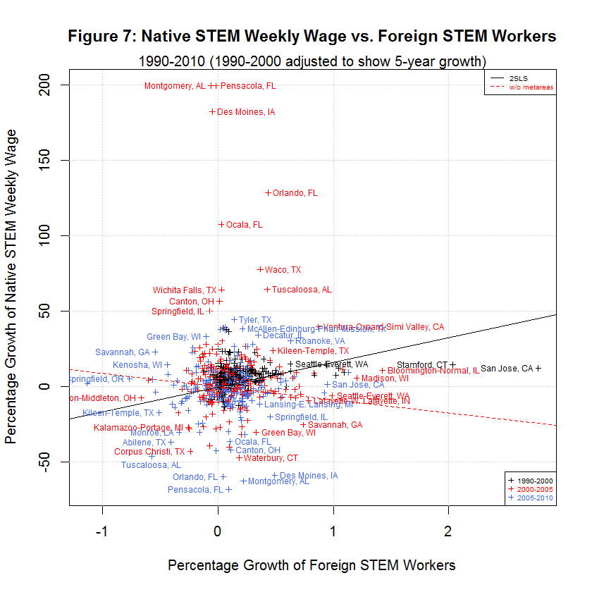
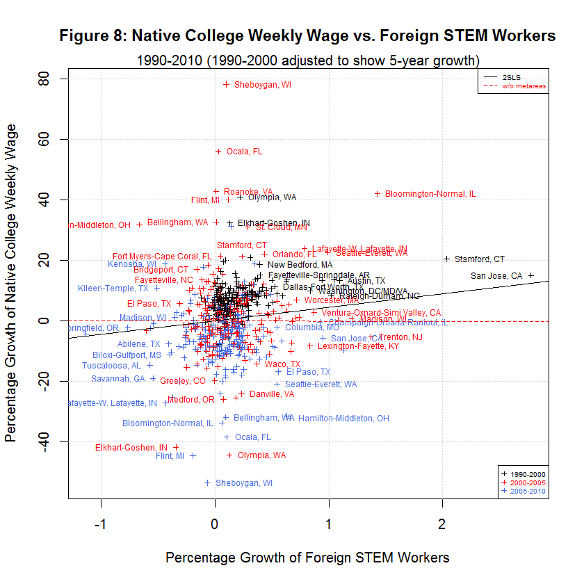
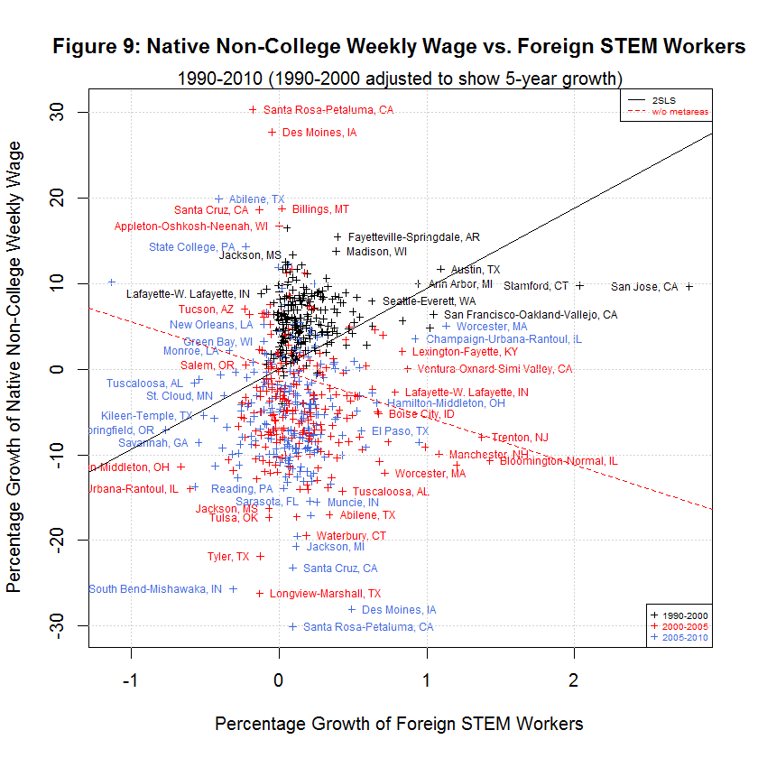
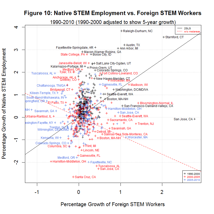
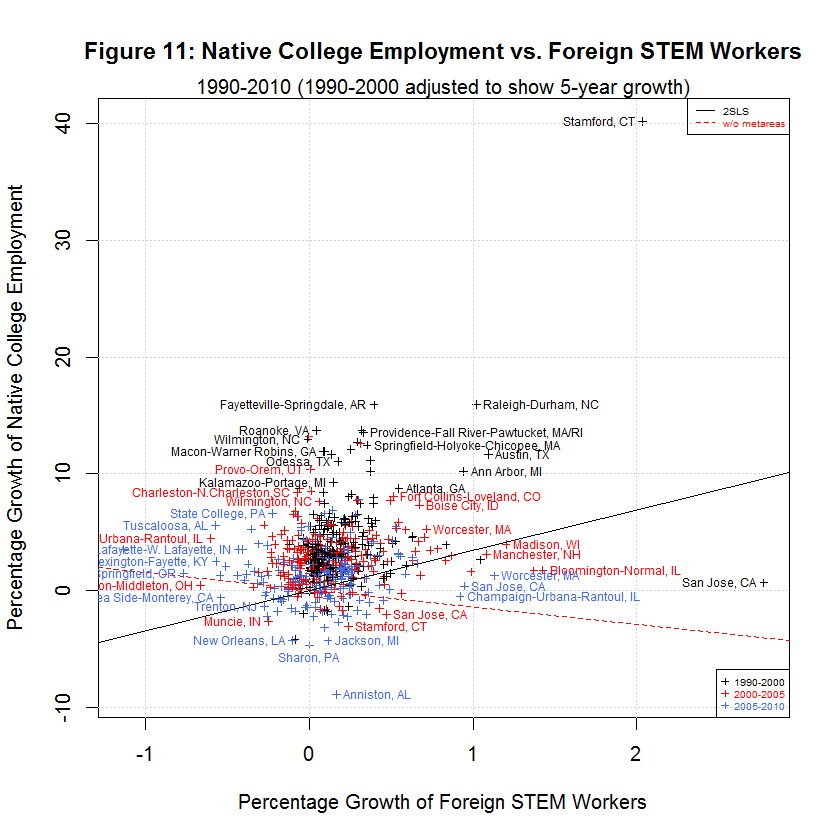
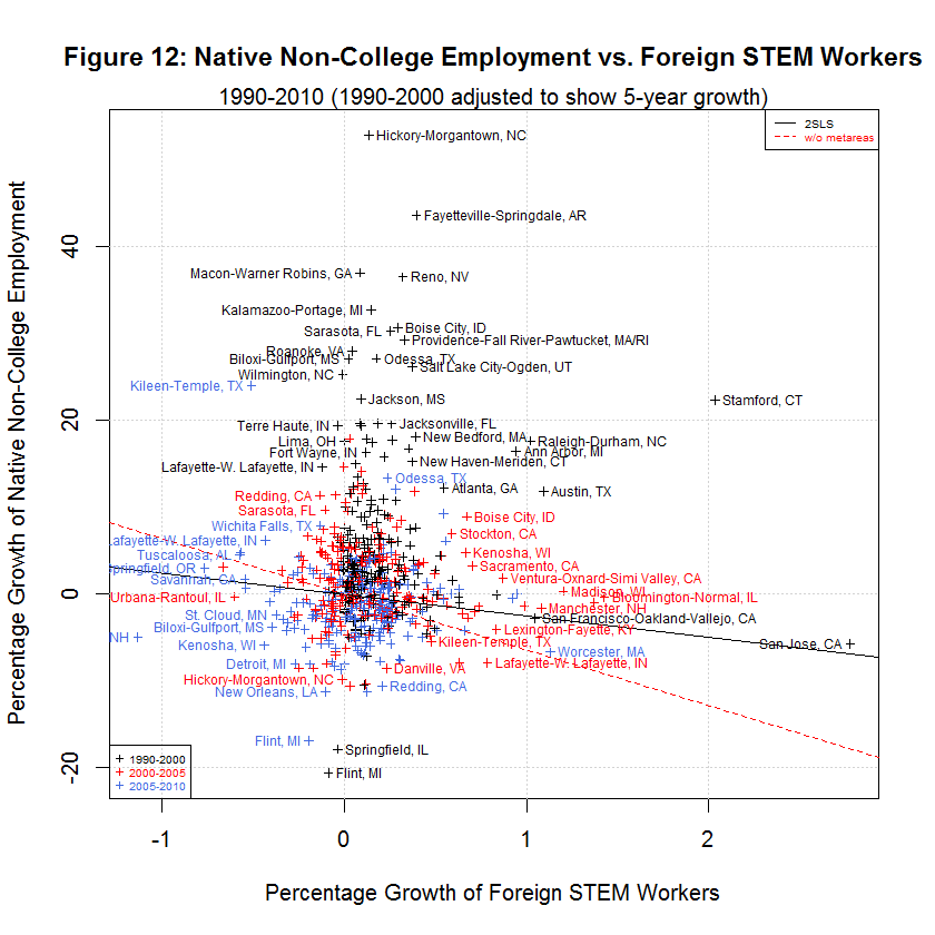
The black lines are the regression lines replicated from the study and the red lines are the regression lines when fmets (representing metareas) is omitted as discussed in a later section. The following table shows the averages of the independent and six dependent variables during the three time spans:
[1] "AVERAGES OF INDEPENDENT AND SIX DEPENDENT VARIABLES IN ORIGINAL AND ADJUSTED DATA"
[1] "                                              "
[1] "      5-YEAR                                  "
[1] "      GROWTH       STUDY'S ORIGINAL DATA      "
[1] "    ---------  -------------------------------"
[1] " N  1990-2000  1990-2000  2000-2005  2005-2010  Variable"
[1] "--  ---------  ---------  ---------  ---------  --------"
[1] " 0)    0.1907     0.3827     0.1375     0.0701  Foreign STEM Workers"
[1] " 1)    7.0068    15.0447     6.9259    -1.2507  Native STEM Weekly Wage"
[1] " 2)    7.2883    15.3769     1.4646    -5.7251  Native College Weekly Wage"
[1] " 3)    5.9075    12.2605    -3.9557    -4.9925  Native Non-College Weekly Wage"
[1] " 4)    0.6605     1.3310     0.0738     0.1278  Native STEM Employment"
[1] " 5)    4.1290     8.5920     2.9037     1.4123  Native College Employment"
[1] " 6)    5.5898    12.3931     1.4488    -1.3758  Native Non-College Employment"
This table is the same as the table shown in the prior table except that the second column from the left has been added to show the 5-year adjusted growth for 1990 to 2000. The other time spans were not adjusted since they are already 5-year spans. The table shows the same general relationship between the three times spans as was the case with the unadjusted data. In general, the growth in native weekly wages and employment was highest in 1990-2000, lower in 2000-2005, and lowest in 2005-2010. However, the difference between 1990-2000 and 2000-2005 is much less now that the data has been properly adjusted. As before, the one exception to the general trend is Native STEM Employment for which the lowest rate was 2000-2005.
7. Resolving the Unequal Time Span Problem by Using Two 10-Year Spans
Another way of resolving the problem of unequal time spans is to use two 10-year time spans, 1990-2000 and 2000-2010. In effect, the data for 2005 is ignored. Following are the coefficients and key numbers for the resulting regressions:
[1] "1990-2010 USING STUDY'S FORMULA AND JUST TWO 10-YEAR SPANS, 1990-2000 AND 2000-2010"
[1] ""
[1] " N  INTERCEPT    SLOPE    STUDY    % DIFF     S.E.   T-STAT    P-VAL  DESCRIPTION"
[1] "--  ---------  --------  -------  -------  -------  -------  -------  -----------------------------------"
[1] " 1)   -0.7210   15.3665   6.6500   131.07    9.627    1.596    0.112  Weekly Wage, Native STEM"
[1] " 2)   -0.0982    3.6908   8.0300   -54.04    5.176    0.713    0.477  Weekly Wage, Native College-Educated"
[1] " 3)   -0.0900    4.2199   3.7800    11.64    2.638    1.599    0.111  Weekly Wage, Native Non-College-Educated"
[1] " 4)    0.0360    0.6472   0.5300    22.11    0.393    1.646    0.101  Employment, Native STEM"
[1] " 5)   -0.0945    3.4955   2.4800    40.95    2.137    1.636    0.103  Employment, Native College-Educated"
[1] " 6)   -0.6489   -0.2329  -5.1700   -95.50    5.078   -0.046    0.963  Employment, Native Non-College-Educated"
As with the previously adjusted data, all of the p-values are now above the minimum significance level reported in the study of 10% (0.100). The following table shows the averages of the independent and six dependent variables during the two 10-year spans:
[1] "AVERAGES OF INDEPENDENT AND SIX DEPENDENT VARIABLES USING 1990-2000 AND 2000-2010"
[1] "                                              "
[1] " N  1990-2000  2000-2010  Variable"
[1] "--  ---------  ---------  --------"
[1] " 0)    0.3827     0.1375  Foreign STEM Workers"
[1] " 1)   15.0447     6.9259  Native STEM Weekly Wage"
[1] " 2)   15.3769     1.4646  Native College Weekly Wage"
[1] " 3)   12.2605    -3.9557  Native Non-College Weekly Wage"
[1] " 4)    1.3310     0.0738  Native STEM Employment"
[1] " 5)    8.5920     2.9037  Native College Employment"
[1] " 6)   12.3931     1.4488  Native Non-College Employment"
As can be seen, all of the growth rates were higher in 1990-2000 than in 2000-2010. The one growth rate that declined was native non-college weekly wage from 2000-2010. Looking at two 10-year spans does have the advantage of making the time spans of equal length such that no adjustment is required. However, it has the disadvantage of dropping a third of the data points in going from three to just two time spans.
8. Looking at Raw Growth Rates Versus the Natural Log of Growth Rates
As mentioned in section 5, following are the results of the regressions after adjusting 1990-2000 to a 5-year growth rate:
[1] "1990-2010 USING STUDY'S FORMULA AND ADJUSTING 1990-2000 TO 5-YEAR GROWTH RATE"
[1] ""
[1] " N  INTERCEPT    SLOPE    STUDY    % DIFF     S.E.   T-STAT    P-VAL  DESCRIPTION"
[1] "--  ---------  --------  -------  -------  -------  -------  -------  -----------------------------------"
[1] " 1)   -0.0816   16.3973   6.6500   146.58   29.129    0.563    0.574  Weekly Wage, Native STEM"
[1] " 2)   -0.0396    4.4957   8.0300   -44.01   14.459    0.311    0.756  Weekly Wage, Native College-Educated"
[1] " 3)    0.0746    9.3902   3.7800   148.42    6.783    1.384    0.167  Weekly Wage, Native Non-College-Educated"
[1] " 4)    0.0066    1.2831   0.5300   142.09    1.010    1.271    0.204  Employment, Native STEM"
[1] " 5)    0.0113    3.4363   2.4800    38.56    3.606    0.953    0.341  Employment, Native College-Educated"
[1] " 6)   -0.0401   -2.4571  -5.1700   -52.47    5.627   -0.437    0.663  Employment, Native Non-College-Educated"
Following are the results of annualizing all of the years to a 1-year time span instead of a 5-year time span:
[1] "1990-2010 USING STUDY'S FORMULA (all years annualized to show 1-year growth)"
[1] ""
[1] " N  INTERCEPT    SLOPE    STUDY    % DIFF     S.E.   T-STAT    P-VAL  DESCRIPTION"
[1] "--  ---------  --------  -------  -------  -------  -------  -------  -----------------------------------"
[1] " 1)   -0.0188    6.2001   6.6500    -6.77   25.966    0.239    0.811  Weekly Wage, Native STEM"
[1] " 2)   -0.0126    3.6896   8.0300   -54.05   14.822    0.249    0.804  Weekly Wage, Native College-Educated"
[1] " 3)    0.0131    9.1280   3.7800   141.48    6.977    1.308    0.191  Weekly Wage, Native Non-College-Educated"
[1] " 4)    0.0012    1.2894   0.5300   143.27    1.019    1.265    0.206  Employment, Native STEM"
[1] " 5)    0.0029    2.8371   2.4800    14.40    3.427    0.828    0.408  Employment, Native College-Educated"
[1] " 6)   -0.0071   -1.9430  -5.1700   -62.42    5.304   -0.366    0.714  Employment, Native Non-College-Educated"
Note that the coefficients, standard errors, t-stats and p-values have all changed. This is despite the fact that the only thing that changed in the data was the period over which the data was annualized. The problem is that, as explained at this link, one should use the logarithm of a growth rate in order to use a linear regression. The reason is because a constant growth rate is exponential but the logarithm of that constant growth rate is linear.
Now, following are the same regression using the natural logarithms of the growth rates rather than the raw growth rates:
[1] "1990-2010 USING STUDY'S FORMULA (all years annualized to show 1-year growth) USING NATURAL LOGS"
[1] ""
[1] " N  INTERCEPT    SLOPE    STUDY    % DIFF     S.E.   T-STAT    P-VAL  DESCRIPTION"
[1] "--  ---------  --------  -------  -------  -------  -------  -------  -----------------------------------"
[1] " 1)   -0.0191    3.9265   6.6500   -40.96   25.884    0.152    0.879  Weekly Wage, Native STEM"
[1] " 2)   -0.0141    3.5317   8.0300   -56.02   15.010    0.235    0.814  Weekly Wage, Native College-Educated"
[1] " 3)    0.0126    9.0611   3.7800   139.71    7.035    1.288    0.198  Weekly Wage, Native Non-College-Educated"
[1] " 4)    0.0012    1.2910   0.5300   143.58    1.021    1.264    0.207  Employment, Native STEM"
[1] " 5)    0.0030    2.7039   2.4800     9.03    3.389    0.798    0.425  Employment, Native College-Educated"
[1] " 6)   -0.0069   -1.8279  -5.1700   -64.64    5.237   -0.349    0.727  Employment, Native Non-College-Educated"
[1] "1990-2010 USING STUDY'S FORMULA (1990-2000 adjusted to show 5-year growth) USING NATURAL LOGS"
[1] ""
[1] " N  INTERCEPT    SLOPE    STUDY    % DIFF     S.E.   T-STAT    P-VAL  DESCRIPTION"
[1] "--  ---------  --------  -------  -------  -------  -------  -------  -----------------------------------"
[1] " 1)   -0.0957    3.9265   6.6500   -40.96   25.884    0.152    0.879  Weekly Wage, Native STEM"
[1] " 2)   -0.0703    3.5317   8.0300   -56.02   15.010    0.235    0.814  Weekly Wage, Native College-Educated"
[1] " 3)    0.0632    9.0611   3.7800   139.71    7.035    1.288    0.198  Weekly Wage, Native Non-College-Educated"
[1] " 4)    0.0061    1.2910   0.5300   143.58    1.021    1.264    0.207  Employment, Native STEM"
[1] " 5)    0.0149    2.7039   2.4800     9.03    3.389    0.798    0.425  Employment, Native College-Educated"
[1] " 6)   -0.0344   -1.8279  -5.1700   -64.64    5.237   -0.349    0.727  Employment, Native Non-College-Educated"
Note that the all of the numbers are now identical except for the intercept. Hence, the length of time over which the data is annualized makes no difference to the key results of linear regressions when one looks at the natural logs of the growth rates. When one looks at the raw growth rates, however, it makes a very big difference. This would allow a researcher to choose whichever period of annualization most agreed with his or her thesis. Hence, to be as accurate as possible, this study should have looked at logarithms of the growth rates, not the raw growth rates.
9. The Use of Metropolitan Areas as a Dummy Variable
The indicator variable metarea is especially concerning. The data consists of values from 3 time spans (1990-2000, 2000-2005, and 2005-2010) taken from 219 metareas (metropolitan areas). In making metarea an indicator or dummy variable, 218 terms with 218 coefficients are added to the equation. In essence, each of the 219 metareas has its own independent coefficient based on a mere three data points. This arguably causes overfitting of the data. To test for this, the CVlm function from the DAAG package was used to do K-fold cross-validation on the second formula. The delta_imm_stemO4_H1B_hat80 instrument had to be omitted because CVlm works on a normal multiple regression. In any case, the attempt to do 3-fold cross validation resulted in the following error message:
Error in model.frame.default(Terms, newdata, na.action = na.action, xlev = object$xlevels) :
  factor fmets has new levels Denver-Boulder, CO, El Paso, TX, Fayetteville, NC, Fresno, CA, Louisville, KY/IN, Modesto, CA, Spokane, WA, Vineland-Milville-Bridgetown, NJ
The attempt to do 10-fold cross validation resulted in the following error message:
Error in model.frame.default(Terms, newdata, na.action = na.action, xlev = object$xlevels) :
  factor fmets has new levels Salem, OR
It appears that this is caused because the "test data" has a metarea not contained in the "training data". That's not surprising since there's only 3 data points per metarea.
The following table shows the results of the regressions using the original data if the metarea is dropped as a dummy variable:
[1] "1990-2010 USING STUDY'S FORMULA MINUS METRO AREAS ON STUDY'S ORIGINAL DATA"
[1] ""
[1] " N  INTERCEPT    SLOPE    STUDY    % DIFF     S.E.   T-STAT    P-VAL   DESCRIPTION"
[1] "--  ---------  --------  -------  -------  -------  -------  -------  -----------------------------------"
[1] "1990-2010 USING STUDY'S FORMULA MINUS METRO AREAS"
[1] " 1)   -0.0391   -0.7414   6.6500  -111.15    6.080   -0.122    0.903  Weekly Wage, Native STEM"
[1] " 2)   -0.0183    3.4605   8.0300   -56.91    3.183    1.087    0.277  Weekly Wage, Native College-Educated"
[1] " 3)   -0.0666   -0.9319   3.7800  -124.65    1.519   -0.613    0.540  Weekly Wage, Native Non-College-Educated"
[1] " 4)    0.0374   -0.2474   0.5300  -146.69    0.303   -0.818    0.414  Employment, Native STEM"
[1] " 5)    0.0760   -0.1770   2.4800  -107.14    1.537   -0.115    0.908  Employment, Native College-Educated"
[1] " 6)   -0.2463   -6.3290  -5.1700    22.42    2.926   -2.163    0.031  Employment, Native Non-College-Educated"
The following table shows the same results using the data in which 1990-2000 has been adjusted to a 5-year growth rate:
[1] "1990-2010 USING STUDY'S FORMULA MINUS METRO AREAS AND ADJUSTING 1990-2000 TO 5-YEAR GROWTH RATE"
[1] ""
[1] " N  INTERCEPT    SLOPE    STUDY    % DIFF     S.E.   T-STAT    P-VAL   DESCRIPTION"
[1] "--  ---------  --------  -------  -------  -------  -------  -------  -----------------------------------"
[1] " 1)    0.0704   -8.7669   6.6500  -231.83   11.424   -0.767    0.443  Weekly Wage, Native STEM"
[1] " 2)   -0.0152   -0.0694   8.0300  -100.86    5.557   -0.012    0.990  Weekly Wage, Native College-Educated"
[1] " 3)   -0.0307   -5.5528   3.7800  -246.90    2.876   -1.931    0.054  Weekly Wage, Native Non-College-Educated"
[1] " 4)    0.0148   -0.8258   0.5300  -255.80    0.456   -1.810    0.071  Employment, Native STEM"
[1] " 5)    0.0536   -1.4843   2.4800  -159.85    1.734   -0.856    0.392  Employment, Native College-Educated"
[1] " 6)   -0.0589   -6.3830  -5.1700    23.46    3.158   -2.021    0.044  Employment, Native Non-College-Educated"
As can be seen, dropping the metarea as a dummy variable causes the slope of the regression to decrease in every case, turning negative in every case with the adjusted data and in all but one case with the original data. As can be seen, the only variables with p-values within the study's minimum significance level of 10% (0.100) are native non-college wages for the adjusted data and native non-college employment for both sets of data. Both now show a negative correlation.
10. A Closer Look at Cross Validation using CVlm
It was found that a value of 20 for the number of folds did work. Following is the first part of the resulting output:
Analysis of Variance Table

Response: delta_native_coll_wkwage
                  Df Sum Sq Mean Sq F value Pr(>F)
delta_imm_stemO4   1   1.45   1.452   80.88 <2e-16 ***
fspan              2   3.87   1.934  107.72 <2e-16 ***
fmets            218   0.63   0.003    0.16   1.00
bartik_coll_wage   1   0.08   0.076    4.22   0.04 *
bartik_coll_emp    1   0.00   0.000    0.02   0.88
Residuals        432   7.75   0.018
---
Signif. codes:  0 ‘***’ 0.001 ‘**’ 0.01 ‘*’ 0.05 ‘.’ 0.1 ‘ ’ 1
This suggests that delta_imm_stemO4 and fspan (the year span represented as a factor) are the most significant variables, followed by bartik_coll_wage. Both bartik_coll_emp and fmets (the metareas represented as a factor) appear to have little significance. Following is the last part of the resulting output:
Overall (Sum over all 32 folds)
    ms
0.0268
I'm not sure the reason this lists 32 folds as 20 folds are listed in the output above it. In any case, this output is described at this link as follows:
Here, at the bottom of the output we get the cross validation residual sums of squares (Overall MS); which is a corrected measure of prediction error averaged across all folds. The function also produces a plot (below) of each fold’s predicted values against the actual outcome variable (y); with each fold a different color.
The next section shows examples of plots generated by CVlm. Regarding the text output, the first part of the output shown above suggests that the significant factors following delta_imm_stemO4 are fspan, bartik_coll_wage, bartik_coll_emp, and fmets in that order. The following table shows the value of Overall MS as each of these factors is removed, starting with the least significant one, for each of the six dependent variables:
[1] "Overall MS (residual sums of squares)"
[1] "====================================="
[1] " native   native   native   native   native   native"
[1] " stemO4   coll     nocoll   stemO4   coll     nocoll"
[1] " wkwage   wkwage   wkwage   emp      emp      emp      TOTAL   regressors"
[1] "-------  -------  -------  -------  -------  -------  -------  ----------"
[1] "0.09465  0.02681  0.00956  0.00017  0.00441  0.02507  0.16067  delta_imm_stemO4 + fspan + fmets + bartik_coll_wage + bartik_coll_emp"
[1] "0.04749  0.01315  0.00477  0.00011  0.00315  0.01747  0.08613  delta_imm_stemO4 + fspan         + bartik_coll_wage + bartik_coll_emp"
[1] "0.04720  0.01302  0.00477  0.00011  0.00316  0.01741  0.08566  delta_imm_stemO4 + fspan         + bartik_coll_wage"
[1] "0.04717  0.01307  0.00480  0.00011  0.00316  0.01734  0.08565  delta_imm_stemO4 + fspan"
[1] "0.05023  0.01899  0.01030  0.00013  0.00371  0.02030  0.10367  delta_imm_stemO4"
As can be seen, the largest residual sum of squares was for the entire formula, including fmets, and the next largest residual sum of squares was for the single regressor delta_imm_stemO4. The residual sums of squares for the other formulas are nearly equal. Judging from the totals, regressors fspan + bartik_coll_wage gives the lowest, fspan by itself gives the next lowest, and fspan + bartik_coll_wage + bartik_coll_emp gives the next lowest. All three of these include the primary regressor delta_imm_stemO4, of course.
In summary, these results suggest that fmets (based on the metareas) is not significant and, in fact, overfits the data. On the other hand, fspan (based on the yearly spans) appears to be significant and does improve the model. Finally, bartik_coll_wage and bartik_coll_emp appear to have little effect on the model, one way or the other.
11. A Look at the Plots Generated by CVlm
Following is the plot produced for native_coll_wkwage with all of the regressors, followed by the plot that is produced if fmets is omitted:
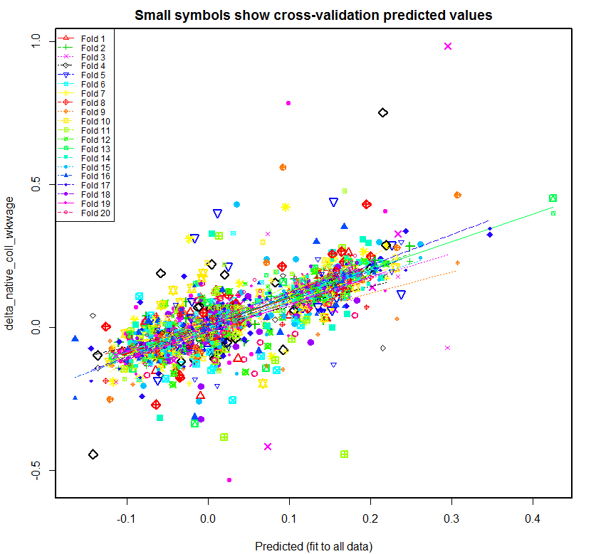
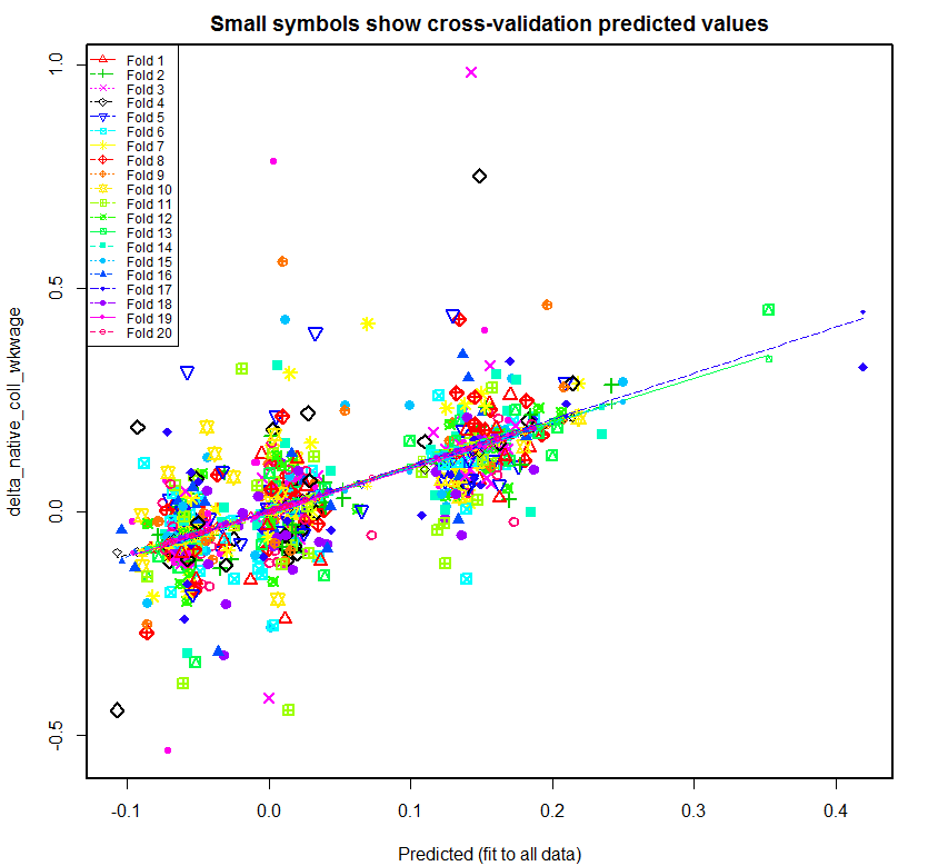
As can be seen, the regression lines created for the 20 folds are much more varied in the first plot. Once fmets is removed as a regressor, the regression lines become more closer to each other. This suggests that this second model is better at predicting new data. Another interesting thing is that the second plot has three fairly distinct clouds of data. This would need additional analysis to verify but it seems likely that these three clouds are related to the three time spans. These graphs correspond to the second dependent variable for Native College-educated Weekly Wage (delta_native_coll_wkwage), shown in the second plot in the next section. As can be seen from that plot, the growth of native college-educated weekly wage was generally highest in 1990-2000, lower in 2000-2005, and lowest in 2005-2010. Hence, the three clouds in the second plot above likely correspond to 1990-2000, 2000-20005, and 2005-2010 from right to left. That is, the growth of weekly wages of college-educated has been generally dropping since 1990-2000.
12. A Look at the Residuals and Plots Generated by CVlm using the New Adjusted Data
The following table shows the value of Overall MS as each of the same five factors as before is removed, starting with the least significant one, for each of the six dependent variables:
[1] "Overall MS (residual sums of squares)"
[1] "====================================="
[1] " native   native   native   native   native   native"
[1] " stemO4   coll     nocoll   stemO4   coll     nocoll"
[1] " wkwage   wkwage   wkwage   emp      emp      emp      TOTAL   regressors"
[1] "-------  -------  -------  -------  -------  -------  -------  ----------"
[1] "0.07806  0.01973  0.00749  0.00010  0.00128  0.00617  0.11284  delta_imm_stemO4 + fspan + fmets + bartik_coll_wage + bartik_coll_emp"
[1] "0.04045  0.00975  0.00364  0.00005  0.00089  0.00446  0.05925  delta_imm_stemO4 + fspan         + bartik_coll_wage + bartik_coll_emp"
[1] "0.04031  0.00969  0.00363  0.00005  0.00090  0.00448  0.05906  delta_imm_stemO4 + fspan         + bartik_coll_wage"
[1] "0.04028  0.00977  0.00366  0.00005  0.00090  0.00447  0.05913  delta_imm_stemO4 + fspan"
[1] "0.04124  0.01231  0.00604  0.00006  0.00099  0.00524  0.06588  delta_imm_stemO4"
Following is the plot produced for native_coll_wkwage with all of the regressors, followed by the plot that is produced if fmets is omitted. Both use the data that is adjusted to account for the differing lengths of time spans as described above.
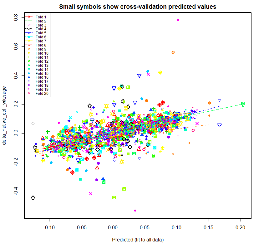
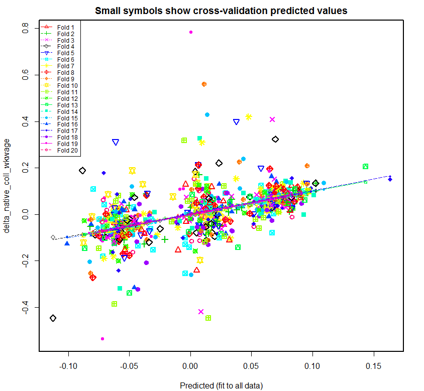
As before, the regression lines created for the 20 folds are much more varied in the first plot. Once fmets is removed as a regressor, the regression lines become more closer to each other, suggesting that this second model is better at predicting new data. Also as before, the second plot has three fairly distinct clouds of data likely related to the three time spans. The main difference from the prior second plot is that the rightmost cloud of data, likely corresponding to 1990-2000, is less separated from the other two clouds as expected.
In summary, there are at least four issues with this study. First there is an apparent typo in one of the numbers (see Section 2). This needs to be fixed.
Secondly, time-spans of different length are combined with no adjustment made for the difference in length (see Sections 5-7). This appears to result in a false correlation and significance in the p-values which disappears when the 10-year growth rate is adjusted to a 5-year growth rate, matching the other two time spans. This is also the case if two 10-year time spans are used.
Thirdly, the study does a linear regression of raw growth rates (see Section 8). This causes the coefficients and key results of the regression to change depending on the length of the time spans or whether the data is annualized. To avoid this, the study should use the logarithms of the growth rates.
Finally, there is a great deal of evidence that the use of metareas as a dummy variable is overfitting the data (see Sections 9-12). This would seem intuitive in that it is adding a coefficient for every metarea even though each metarea contains only three data points. In addition, a test of the data with cross validation provides strong evidence that the use a metarea dummy variable is overfitting and giving false results.
14. Replicating the Above Results
Following are the instructions that I received from the Journal of Labor Economics on obtaining the data required to replicate the study:
Go to the listing at http://www.jstor.org/stable/10.1086/679275 and click on the article. Just above the title, you will see four choices. The fourth one is a pull-down menu labeled “Supplements.” When you click on this menu, you will see six data files.
These files can be unzipped into a directory structure in which the file PSS_Data.dta is at the following location:
13042data\JOLE Data & Do Files\JOLE_regressions_tables\PSS_Data.dtaThe R program jole_pss_tab5.R listed below reads PSS_Data.dta from this location and produces the results given in this analysis. It also reads the following csv files in order to create and label the first twelve plots. However, it should be noted that PSS_Data.dta is not data from the original source. It is data calculated by the study from the original source. The next section deals with the replication and verification of the data in PSS_Data.dta.
Source Code for R Programs and Data Files Used in this Analysis