OCC1990 is a modified version of the 1990 Census Bureau occupational classification scheme. OCC1990 provides researchers with a consistent classification of occupations using the 1990 coding scheme as its starting point. It spans the period from 1950 forward.
Following is a list of the extracted variables, including those for the years of 1980, 1990, 2000, 2010, and 2017:
                                                                  2017 2010 2000 1990 1980
Variable    Variable Label                            Type  Codes  acs  acs 5pct 5pct 5pct
----------  ----------------------------------------- ----  ----- ---- ---- ---- ---- ----
YEAR        Census year [preselected].................. H   codes   X    X    X    X    X
DATANUM     Data set number [preselected].............. H   codes   X    X    X    X    X
SERIAL      Household serial number [preselected]...... H   codes   X    X    X    X    X
CBSERIAL    Original CB household serial number [pre].. H   codes   X    X    .    .    .
HHWT        Household weight [preselected]............. H   codes   X    X    X    X    X
GQ          Group quarters status [preselected]........ H   codes   X    X    X    X    X
PERNUM      Person number in sample unit [preselected]. P   codes   X    X    X    X    X
PERWT       Person weight [preselected]................ P   codes   X    X    X    X    X
STATEFIP    State (FIPS code).......................... H   codes   X    X    X    X    X
COUNTYFIP   County (FIPS code)......................... H   codes   X    X    X    X    X
MET2013     Metropolitan area (2013 OMB delineations).. H   codes   X    X    X    .    .
PUMA        Public Use Microdata Area.................. H   codes   X    X    X    X    .
SEX         Sex........................................ P   codes   X    X    X    X    X
AGE         Age........................................ P   codes   X    X    X    X    X
RACE        Race....................................... P   codes   X    X    X    X    X
HISPAN      Hispanic origin............................ P   codes   X    X    X    X    X
BPL         Birthplace................................. P   codes   X    X    X    X    X
CITIZEN     Citizenship status......................... P   codes   X    X    X    X    X
YRIMMIG     Year of immigration........................ P   codes   X    X    X    X    X
EDUC        Educational attainment..................... P   codes   X    X    X    X    X
DEGFIELD    Field of degree............................ P   codes   X    X    .    .    .
DEGFIELD2   Field of degree (2)........................ P   codes   X    X    .    .    .
EMPSTAT     Employment status.......................... P   codes   X    X    X    X    X
OCC         Occupation................................. P   codes   X    X    X    X    X
OCC1990     Occupation, 1990 basis..................... P   codes   X    X    X    X    X
CLASSWKR    Class of worker............................ P   codes   X    X    X    X    X
WKSWORK2    Weeks worked last year, intervalled........ P   codes   X    X    X    X    X
INCWAGE     Wage and salary income..................... P   codes   X    X    X    X    X
Due to memory constraints, the current online version of the app only includes 2010 and 2017 at present. This may be expanded in the future. Still, since the online app currently includes just two years, this document will focus mainly on looking at a single year's data.
From the variables listed above, RACE, HISPAN, BPL, EDUC, DEGFIELD, DEGFIELD2, EMPSTAT, and CLASSWKR each include an additional detailed variable with the same name with a D added. For example RACE will have a detailed version named RACED. Hence, the 28 variable selected for 2017 above will actually result in 36 variables, including the 8 detailed variables. Following are detailed descriptions of all of these variables:
p YEAR     : int  sample year: currently 2014 to 2017
p DATANUM  : int  particular sample from which the case is drawn in a given year. See DATANUM Codes
p SERIAL   : int  identifying number unique to each household record in a given sample.
p CBSERIAL : num  unique, original identification number assigned to each household record in a given sample by the Census Bureau.
p HHWT     : int  indicates how many households in the U.S. population are represented by a given household in an IPUMS sample.
p GQ       : int  classifies all housing units as a vacant units (0), households (1-2), or group quarters (3-5). See GQ Codes
p PERNUM   : int  numbers all persons within each household consecutively in the order in which they appear on the original census or survey form.
p PERWT    : int  indicates how many persons in the U.S. population are represented by a given person in an IPUMS sample.
# STATEFIP : int  state where the household was located, using the FIPS coding scheme. See STATEFIP Codes
# COUNTY   : int  county where the household was located, using the ICPSR coding scheme (renamed COUNTYFIP). See COUNTY Codes
# MET2013  : int  metro area where the household was located, using the 2013 definitions for metropolitan statistical areas (MSAs) from the OMB. See MET2013 Codes
# PUMA     : int  identifies the Public Use Microdata Area (PUMA) where the housing unit was located. See PUMA Codes
# SEX      : int  1 = male, 2 = female
# AGE      : int  age in years, 0 = Less than 1 year old, 96 = maximum in 2017
# RACE     : int  race, 1 = White, 2 = Black, 3 = American Indian or Alaskan Native, 4 = Chinese, 5 = Japanese, 6 = Other Asian or Pacific Islander, 7 = Other race, 8 = Two major races, 9 = Three or more major races
a RACED    : int  detailed race, 100 to 996, see RACE Codes
# HISPAN   : int  Hispanic origin, 0 = Not Hispanic, 1 = Mexican, 2 = Puerto Rican, 3 = Cuban, 4 = Other, 9 = Not Reported
a HISPAND  : int  detailed Hispanic origin, 000 to 900, see HISPAN Codes
# BPL      : int  U.S. state or territory or the foreign country where the person was born (188 categories). See BPL Codes
a BPLD     : int  U.S. state or territory or the foreign country where the person was born (572 categories). See BPL Codes
# CITIZEN  : int  citizenship status: 0 = N/A (Born in U.S.), 1 = Born abroad of American parents, 2 = Naturalized citizen, 3 = Not a citizen
# YRIMMIG  : int  year in which a foreign-born person entered the United States. See YRIMMIG Codes
# EDUC     : int  respondents' educational attainment, as measured by the highest year of school or degree completed (12 categories). See EDUC Codes
a EDUCD    : int  respondents' educational attainment, as measured by the highest year of school or degree completed (44 categories). See EDUC Codes
# DEGFIELD : int  field of degree, 00 = N/A, 11 = Agriculture, ... 21 = Computer and Information Sciences, ... 24 = Engineering, 25 = Engineering Technologies, ... 37 = Mathematics and Statistics, ..., 62 = Business, 64 = History
a DEGFIELDD: int  detailed field of degree, 0000 to 6403, see DEGFIELD Codes
# DEGFIELD2: int  second field of study, same codes as DEGFIELD above
a DEGFIELD2D:int  detailed second field of study, same codes as DEGFIELDD above
# EMPSTAT  : int  employment status: 0 = N/A, 1 = Employed, 2 = Unemployed, 3 = Not in labor force
a EMPSTATD : int  employment status: 00 = N/A, 10 = At work, 12 = Has job, not working, 14 = Armed forces--at work, 15 = Armed forces--with job but not at work, 20 = Unemployed, 30 = Not in Labor Force
# OCC      : int  person's primary occupation, coded into a contemporary census classification scheme. See OCC Codes and ACS Occupation Codes
# OCC1990  : int  person's primary occupation, coded to be comparable back to 1950. See OCC1990 Codes and 1990 Occupation Codes
# CLASSWKR : int  worker class: 0 = N/A, 1 = Self-employed, 2 = Works for wages
a CLASSWKRD: int  worker class: 00 = N/A, 13 = Self-employed, not incorporated, 14 = Self-employed, incorporated, 22 = Wage, private, 23 = Wage at non-profit, 25 = Federal government, 27 = State government, 28 = Local government, 29 = Unpaid family worker
# WKSWORK2 : int  number of weeks worked the previous year: 0 = N/A (or Missing), 1 = 1-13 weeks, 2 = 14-26 weeks, 3 = 27-39 weeks, 4 = 40-47 weeks, 5 = 48-49 weeks, 6 = 50-52 weeks
# INCWAGE  : int  total pre-tax wage and salary income in current dollars for the previous year. See INCWAGE Codes
c STATE    : chr  Two-character state abbreviation from https://www2.census.gov/geo/docs/reference/state.txt.
c COUNTY   : chr  County name and two-character state abbreviation from https://www2.census.gov/geo/docs/reference/codes/files/national_county.txt.
c METRO    : chr  Metropolitan area name from https://www2.census.gov/programs-surveys/metro-micro/geographies/reference-files/2017/delineation-files/list2.xls.

# = selected, p = preselected, a = added automatically, c = created from lookups
The # symbol denotes the variables that were manually selected and the p and a symbols that were automatically preselected or selected in response to the manual selections. The last three variables marked with the symbol c were created by using the STATEFIP, COUNTY, and MET2013 to look up the text representations of states, counties, and metropolitan areas in the indicated files.
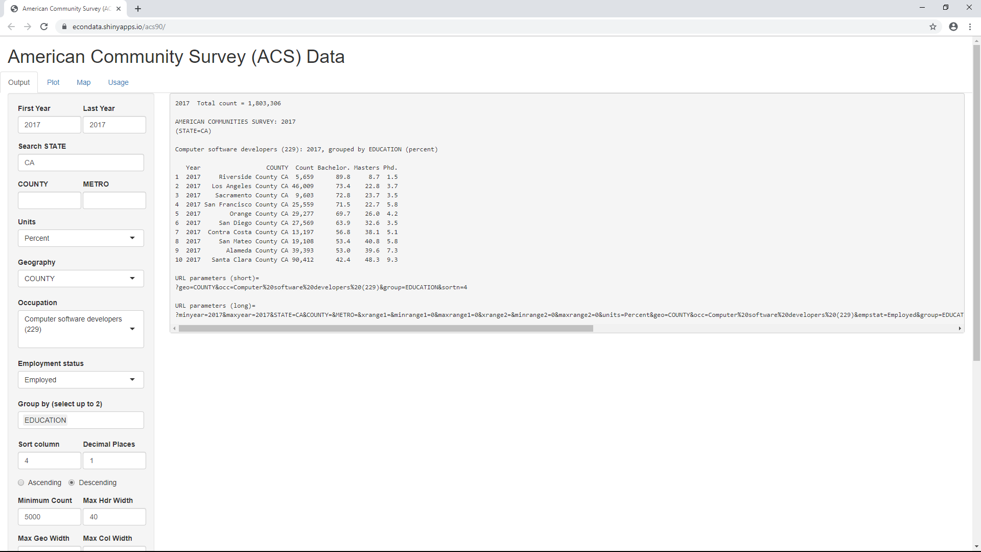
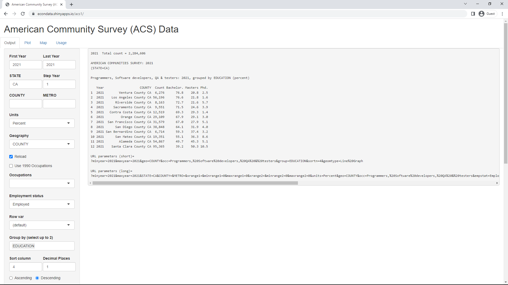
When the acs1 application first starts, it defaults to the following screen:
As can be seen, the screen has four tabs (Output, Plot, Map, and Usage) and is initially set to the Output tab. It displays a table that shows the education level in 2017 of workers with the occupation "Computer software developers (229)" in all counties of California with 5000 or more workers. The format and contents of the table are determined by the default input in the left sidepanel:
Input Label                 Default     Description
--------------------------  ----------  -----------
First Year                  2017        First year to include in data
Last Year                   2017        Last year to include in data
Search STATE                CA          2-character state abbreviation (blank indicates entire U.S.)
COUNTY                                  Optional pattern to match in COUNTY
METRO                                   Optional pattern to match in METRO
Units                       Percent     Count, Percent, or Percent in group (first of two selected groups)
Geography                   COUNTY      STATE, COUNTY, METRO, NATION
Occupation                  Computer software developers (229) - OCC1990 occupation. See OCC1990 Codes and 1990 Occupation Codes
Employment status           Employed    All, Employed, Unemployed, In labor force
Group by (select up to 2)   EDUCATION   Up to two groups for grouping data. Each group is actually a recode for one variable with defined labels for each category within the group.
Sort column                 4           The column by which to sort the rows.
Decimal Places              1           The number of decimals used in percent units.
Ascending/Descending        Descending  The order in which to sort the column specified in "Sort column".
Minimum Count               5000        Minimum count to include in the results.
Max Hdr Width               40
Max Geo Width               40
Max Col Width               40
Maximum Total Width         240
Maximum Total Rows          900
Range field1
Minimum range1              0
Maximum range1              0
Range field2
Minimum range2              0
Maximum range2              0
Ignore URL Parameters
The inputs labelled 'Search STATE', 'COUNTY', and 'METRO' can be used to filter these fields. Hence, the CA in the 'Select STATE' input causes only metro areas in California to be displayed. The data is also filtered by the selection of 5000 in the input labelled 'Minimum Count'. This causes only those metro areas with 5,000 or more of the specified workers to be listed.
The input labelled 'Occupation' can be set to the major occupation groups shown at this link which are in the data. The data for the acs1 application is currently limited to this subset of occupations due to memory issues on the server but may be expanded if possible. The occupation select list also includes some subgroups of these major groups such as "Computer software developers (229). That is what the occupation is set to by default.
The input labelled "Employment status' can be set to filter the workers shown. It can be currently set to 'All', 'Employed', 'Unemployed', and 'In labor force'. This last selection includes all workers, including those not in the labor force.
The input labelled 'Group by' is the key way of selecting the columns for the table. In this case, the columns are obtained by grouping the workers by their education level (EDUCATION). The categories for EDUCATION are "Bachelor-", Masters", and "Phd+" to indicate workers with a Bachelor's degree or less, a Master's degree, or a Phd degree or higher. The third column with the header 'Count' will always contain the total count for the columns to the right of it.
In the default output, the fourth column and up contain percentages of the total count for each column. Hence, these numbers will add up to 100 percent, discounting any round-off error. This output of percents is set by the input labelled 'Units' which is set to 'Percent'. Setting this to 'Percent in group' will have a different affect if the 'Group by' input contains more than one selection. Selecting 'Count' for units will change the output of these columns to the actual counts. Then, their sum will add up to the total count shown in the third column.
The input labelled 'Sort column' specifies the column by which the rows should be sorted. Since it's set to 4, the rows are sorted by the fourth column. Setting it to a minus number counts the columns from the right. Hence, a setting it to -1 causes the rows to be sorted by the last column. The radio buttons labelled 'Ascending' and 'Descending' beneath this input will cause the sorting to be ascending or descending, respectively. Finally, the input labelled 'Decimal places' will set the number of decimals to use when the units is in percents. For units of 'Count', no decimal places are required.
Below the table are shown the URL parameters which can be used to obtain this page, along with the inputs. Since no parameters are listed for the short format, this page can be obtained via a URL https://econdata.shinyapps.io/acs17/. The long format lists all of the parameters and can be copied to make a record of all of the inputs, even the defaults. However, this link could likewise be obtained using these parameters. Note: The parameters may not have been updated to include all possible parameters but will likely be updated to include them soon.
Selecting the Plot tab, will display the following plot:
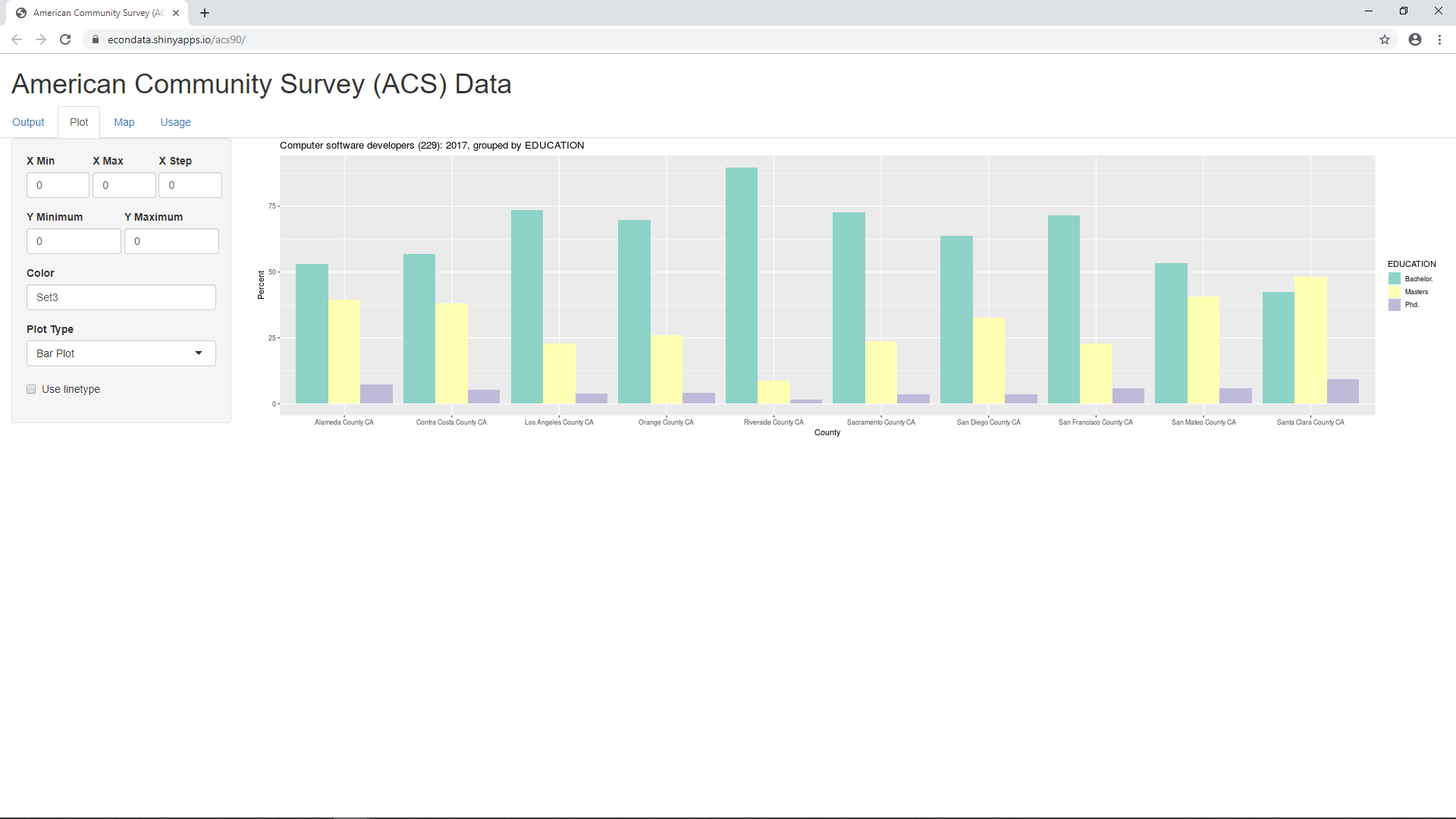
Currently, the "Plot Type" can be set to "Bar Plot" or "Line Graph".
Selecting the Map tab, will display the following plot:
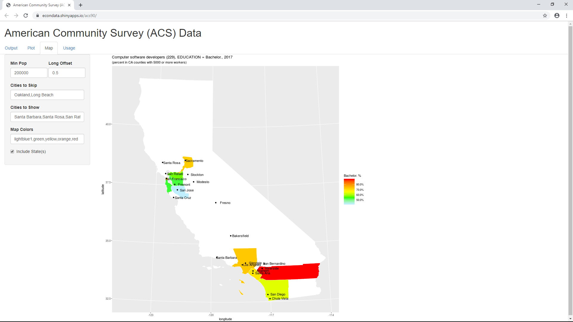
This map corresponds to the following data shown on the Output tab:
   Year                  COUNTY  Count Bachelor. Masters Phd.
1  2017     Riverside County CA  5,659      89.8     8.7  1.5
2  2017   Los Angeles County CA 46,009      73.4    22.8  3.7
3  2017    Sacramento County CA  9,603      72.8    23.7  3.5
4  2017 San Francisco County CA 25,559      71.5    22.7  5.8
5  2017        Orange County CA 29,277      69.7    26.0  4.2
6  2017     San Diego County CA 27,569      63.9    32.6  3.5
7  2017  Contra Costa County CA 13,197      56.8    38.1  5.1
8  2017     San Mateo County CA 19,108      53.4    40.8  5.8
9  2017       Alameda County CA 39,393      53.0    39.6  7.3
10 2017   Santa Clara County CA 90,412      42.4    48.3  9.3
As can be seen, Riverside County ia red since 89.8 percent of its software developers have Bachelor's degrees or less. Los Angeles, Sacramento, San Francisco, and Orange counties are orange since the percentage of their software developers with a Bachelor's degree or less is 73.4, 72.8, 71.5, and 69.7, respectively. San Diego County is yellow-green since its percentage is 63.9 percent and Contra Costa, San Mateo, and Alameda counties are green with percentages of 56.8, 53.4, and 53.0, respectively. Finally, Santa Clara County is light blue since only 42.4 of its software developers have Bachelor's degrees or less.
You can look at counties with just 1,000 or more software developers by going to the Output tab and changing "Minimum Count" to 1000. This will expand the number of counties from 10 to 25 (including (NA) for records for which no county was specified). Clicking the "Ascending" radio button will then display the following rows, sorted from the lowest to highest values of Bachelor's degrees or less:
   Year                    COUNTY  Count Bachelor. Masters Phd.
1  2017     Santa Clara County CA 90,412      42.4    48.3  9.3
2  2017      Santa Cruz County CA  2,342      46.9    33.5 19.6
3  2017         Alameda County CA 39,393      53.0    39.6  7.3
4  2017       San Mateo County CA 19,108      53.4    40.8  5.8
5  2017      Stanislaus County CA  1,075      55.0    34.8 10.2
6  2017    Contra Costa County CA 13,197      56.8    38.1  5.1
7  2017     San Joaquin County CA  2,148      58.7    38.9  2.4
8  2017       San Diego County CA 27,569      63.9    32.6  3.5
9  2017  San Bernardino County CA  4,067      65.5    23.9 10.6
10 2017           Marin County CA  1,579      67.7    32.3  0.0
11 2017          Orange County CA 29,277      69.7    26.0  4.2
12 2017   San Francisco County CA 25,559      71.5    22.7  5.8
13 2017   Santa Barbara County CA  2,208      71.9    13.9 14.2
14 2017      Sacramento County CA  9,603      72.8    23.7  3.5
15 2017     Los Angeles County CA 46,009      73.4    22.8  3.7
16 2017            Yolo County CA  1,016      73.9    26.1  0.0
17 2017 San Luis Obispo County CA  2,394      76.4    23.6  0.0
18 2017         Ventura County CA  3,917      80.9    15.7  3.4
19 2017                      (NA)  2,529      82.2    15.3  2.5
20 2017       El Dorado County CA  1,205      86.4    13.6  0.0
21 2017          Fresno County CA  1,481      86.7    13.3  0.0
22 2017          Placer County CA  2,372      89.0     9.3  1.7
23 2017       Riverside County CA  5,659      89.8     8.7  1.5
24 2017          Sonoma County CA  2,689      94.1     5.9  0.0
25 2017            Kern County CA  1,011     100.0     0.0  0.0
Going back to the Map tab then shows the following map:
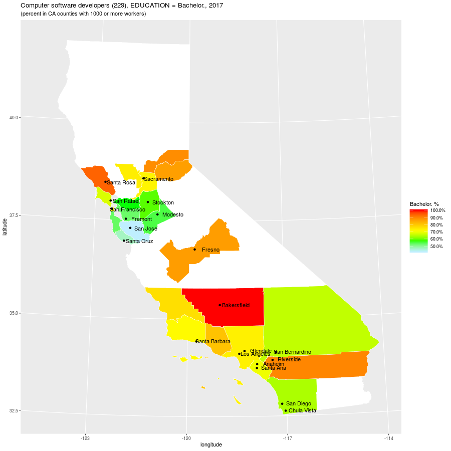
As can be seen, more counties are now colored. Also, the range of the color legend has now changed since the percentages now range from 100.0 to 42.4 percent rather than from 89.8 to 42.4 percent as before. As a result, Riverside County is now brown instead of red and it is Kern County that is red.
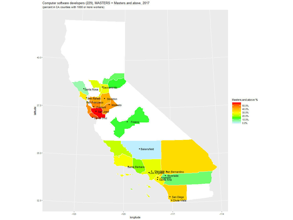
One problem with the above map and table is that they are focused on the percentage of software developers who have a Bachelor's degree or less rather than a Master's degree or more. This is because the program is currently coded to focus on any one category of a currently defined grouping and the EDUCATION grouping has the categories Bachelor (and below), Masters, and Phd (and above). It would likely be clearer and more positive to focus on the latter. This was accomplished by creating a new grouping called Masters with the categories Bachelor and below and Masters and above. Then switching to the Output tab, setting "Group by" to MASTERS and changing "Sort column" to 5 (to select the Masters or above category) will output the following table:
   Year                    COUNTY  Count Bachelor.and.below Masters.and.above
1  2017     Santa Clara County CA 90,412               42.4              57.6
2  2017      Santa Cruz County CA  2,342               46.9              53.1
3  2017         Alameda County CA 39,393               53.0              47.0
4  2017       San Mateo County CA 19,108               53.4              46.6
5  2017      Stanislaus County CA  1,075               55.0              45.0
6  2017    Contra Costa County CA 13,197               56.8              43.2
7  2017     San Joaquin County CA  2,148               58.7              41.3
8  2017       San Diego County CA 27,569               63.9              36.1
9  2017  San Bernardino County CA  4,067               65.5              34.5
10 2017           Marin County CA  1,579               67.7              32.3
11 2017          Orange County CA 29,277               69.7              30.3
12 2017   San Francisco County CA 25,559               71.5              28.5
13 2017   Santa Barbara County CA  2,208               71.9              28.1
14 2017      Sacramento County CA  9,603               72.8              27.2
15 2017     Los Angeles County CA 46,009               73.4              26.6
16 2017            Yolo County CA  1,016               73.9              26.1
17 2017 San Luis Obispo County CA  2,394               76.4              23.6
18 2017         Ventura County CA  3,917               80.9              19.1
19 2017                      (NA)  2,529               82.2              17.8
20 2017       El Dorado County CA  1,205               86.4              13.6
21 2017          Fresno County CA  1,481               86.7              13.3
22 2017          Placer County CA  2,372               89.0              11.0
23 2017       Riverside County CA  5,659               89.8              10.2
24 2017          Sonoma County CA  2,689               94.1               5.9
25 2017            Kern County CA  1,011              100.0               0.0
Switching to the Map tab will then display the following map:
This is likely much more clear as it focuses on the percentage of software developers with a Master's degree and above. In any case, the precise appearance of the prior maps is affected by the values of the inputs following inputs in the left sidepanel:
Input Label         Default                                         Description
------------------  ----------------------------------------------  -----------
Min Pop             200000                                          Minimum population of cities to display. Lowering this will increase the number of cities displayed.
Long Offset         0.5                                             This will set the approximate offset to the left of the city dot that the city name will appear (in units of longitude).
Cities to Skip      Oakland,Long Beach                              This default for California suppressed the display of Oakland and Long Beach which overwrote other city names.
Cities to Show      Santa Barbara,Santa Rosa,San Rafael,Santa Cruz  This default for California adds additional cities which have less than the population specified by "Min Pop"
Map Colors          lightblue1,green,yellow,orange,red              This sets the range of colors used.
Include State(s)    True(checked)                                   This will cause the entire state (or states for a U.S. map) to display. If unchecked, only the specified counties are displayed.
Going back to the Output tab, blanking out the "Search State" field, and returning to the Map tab will display the following map of the entire United States:
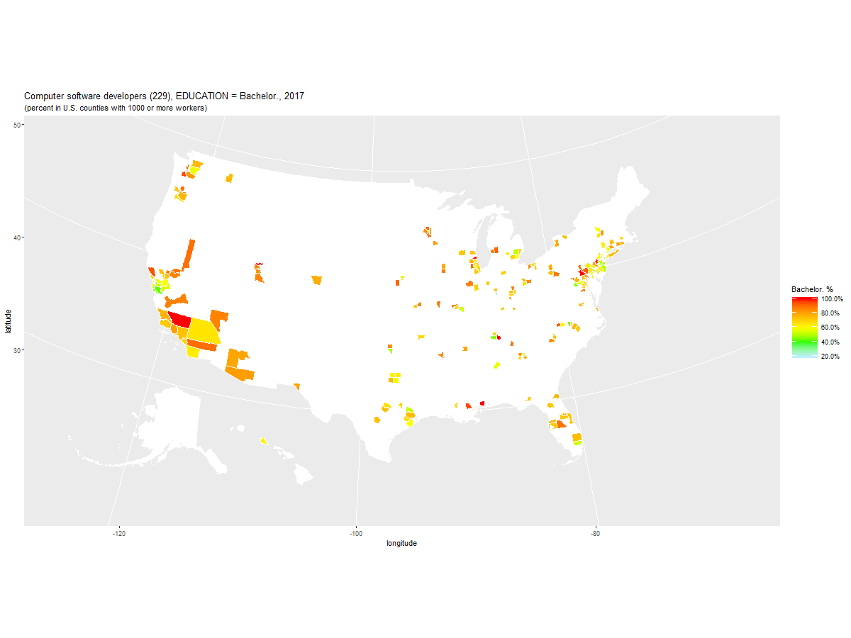
As can be seen, most of the counties are colored white. This is because they contain less than 1000 software developers as determined by the survey. Fortunately, it's also possible to look at the percentages by state. Go back to the Output tab and change "Geography" to STATE. This will display a table of 49 of the 50 states plus Washington D.C. To get the missing two states, change "Minimum Count" to 500. The following table of all 50 states plus Washing D.C. will display:
   Year STATE   Count Bachelor. Masters Phd.
1  2017    ME   3,541      92.3     7.7  0.0
2  2017    MS   4,546      92.3     4.9  2.8
3  2017    AK     806      91.9     8.1  0.0
4  2017    ID   5,281      90.6     9.4  0.0
5  2017    VT   2,563      89.4    10.6  0.0
6  2017    ND   1,623      88.8    11.2  0.0
7  2017    NV   6,256      87.5     9.6  3.0
8  2017    UT  27,182      85.3    12.0  2.7
9  2017    IA  14,940      85.0    12.7  2.3
10 2017    SD   1,739      82.9    17.1  0.0
11 2017    MO  24,758      82.6    16.4  1.0
12 2017    KY  14,512      82.2    17.1  0.6
13 2017    LA   7,395      81.0    16.5  2.5
14 2017    AZ  28,209      80.2    18.7  1.1
15 2017    MN  40,479      80.1    19.6  0.3
16 2017    SC  14,240      79.2    18.9  1.8
17 2017    AR   9,064      78.5    19.1  2.4
18 2017    WI  29,884      78.3    20.1  1.6
19 2017    OR  25,863      77.4    18.7  3.9
20 2017    AL  16,830      76.4    21.4  2.2
21 2017    OK   9,088      76.2    21.7  2.1
22 2017    NE  10,468      74.8    24.3  0.9
23 2017    IN  20,973      74.8    25.0  0.2
24 2017    TN  22,638      74.6    23.2  2.2
25 2017    WY     877      74.5     0.0 25.5
26 2017    CT  18,030      74.1    21.6  4.3
27 2017    RI   5,858      74.0    23.6  2.3
28 2017    PA  62,516      73.9    23.6  2.5
29 2017    OH  44,869      73.9    24.2  2.0
30 2017    NC  54,871      72.8    24.3  2.9
31 2017    FL  73,765      72.6    24.1  3.3
32 2017    KS  14,361      71.7    25.1  3.2
33 2017    NH  13,140      71.6    26.2  2.3
34 2017    WV   2,847      71.4    28.6  0.0
35 2017    GA  51,081      70.7    28.3  1.1
36 2017    HI   2,935      70.1    25.5  4.4
37 2017    IL  66,867      69.5    26.3  4.2
38 2017    CO  50,474      69.4    27.9  2.7
39 2017    TX 133,351      68.2    29.0  2.8
40 2017    NY  92,198      68.0    28.4  3.6
41 2017    MT   2,241      67.5    20.9 11.6
42 2017    MI  41,988      66.5    32.6  0.9
43 2017    MD  58,240      66.0    30.7  3.4
44 2017    NM   5,047      64.3    29.5  6.2
45 2017    WA  94,231      63.5    31.4  5.1
46 2017    MA  70,723      62.6    30.2  7.2
47 2017    VA  78,219      60.7    35.3  3.9
48 2017    CA 340,950      60.2    33.8  6.0
49 2017    NJ  70,269      57.1    39.1  3.9
50 2017    DE   3,662      56.0    36.6  7.3
51 2017    DC   6,818      49.4    47.6  2.9
As can be seen Alaska (AK) and Wyoming (WY) had 806 and 877 software developers in 2017, respectively. Going back to the Map tab will display the following map of the entire United States:
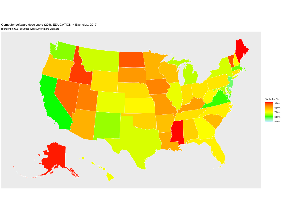
As can be seen, all of the states are colored according to the percentage of its software developers who have a Bachelor's degree or less. Of course, Alaska and Wyoming would have been white if "Minimum Count" had been left set to 1,000. Still, it does seem to be more useful to look at a relatively small population, like software developers, by state when looking at the entire United States.
2021 Updated Documentation
In 2001, the variable DATANUM was changed to SAMPLE and the automatic variables CLUSTER and STRATA were added. Also, the variables PREDHISP and POVERTY were added to the variables being extracted in 2019. Following are detailed descriptions of all of the current variables as of 2021:
H YEAR     : int  sample year: currently 2014 to 2017
H SAMPLE   : int  IPUMS sample identifier. See SAMPLE Codes
H SERIAL   : int  identifying number unique to each household record in a given sample.
H CBSERIAL : num  unique, original identification number assigned to each household record in a given sample by the Census Bureau.
H HHWT     : int  indicates how many households in the U.S. population are represented by a given household in an IPUMS sample.
H CLUSTER  : int  Household cluster for variance estimation.
H STATEFIP : int  state where the household was located, using the FIPS coding scheme. See STATEFIP Codes
H COUNTYFIP: int  county where the household was located, using the ICPSR coding scheme (renamed COUNTYFIP). See COUNTY Codes
H MET2013  : int  metro area where the household was located, using the 2013 definitions for metropolitan statistical areas (MSAs) from the OMB. See MET2013 Codes
H PUMA     : int  identifies the Public Use Microdata Area (PUMA) where the housing unit was located. See PUMA Codes
H STRATA   : int  Household strata for variance estimation.
H GQ       : int  classifies all housing units as a vacant units (0), households (1-2), or group quarters (3-5). See GQ Codes
P PERNUM   : int  numbers all persons within each household consecutively in the order in which they appear on the original census or survey form.
P PERWT    : int  indicates how many persons in the U.S. population are represented by a given person in an IPUMS sample.
P SEX      : int  1 = male, 2 = female
P AGE      : int  age in years, 0 = Less than 1 year old, 96 = maximum in 2017
P RACE     : int  race, 1 = White, 2 = Black, 3 = American Indian or Alaskan Native, 4 = Chinese, 5 = Japanese, 6 = Other Asian or Pacific Islander, 7 = Other race, 8 = Two major races, 9 = Three or more major races
P RACED    : int  detailed race, 100 to 996, see RACE Codes
P HISPAN   : int  Hispanic origin, 0 = Not Hispanic, 1 = Mexican, 2 = Puerto Rican, 3 = Cuban, 4 = Other, 9 = Not Reported
P HISPAND  : int  detailed Hispanic origin, 000 to 900, see HISPAN Codes
P BPL      : int  U.S. state or territory or the foreign country where the person was born (188 categories). See BPL Codes
P BPLD     : int  U.S. state or territory or the foreign country where the person was born (572 categories). See BPL Codes
P CITIZEN  : int  citizenship status: 0 = N/A (Born in U.S.), 1 = Born abroad of American parents, 2 = Naturalized citizen, 3 = Not a citizen
P YRIMMIG  : int  year in which a foreign-born person entered the United States. See YRIMMIG Codes
P PREDHISP : Hispanic/Latino response predicted value.
P EDUC     : int  respondents' educational attainment, as measured by the highest year of school or degree completed (12 categories). See EDUC Codes
P EDUCD    : int  respondents' educational attainment, as measured by the highest year of school or degree completed (44 categories). See EDUC Codes
P DEGFIELD : int  field of degree, 00 = N/A, 11 = Agriculture, ... 21 = Computer and Information Sciences, ... 24 = Engineering, 25 = Engineering Technologies, ... 37 = Mathematics and Statistics, ..., 62 = Business, 64 = History
P DEGFIELDD: int  detailed field of degree, 0000 to 6403, see DEGFIELD Codes
P DEGFIELD2: int  second field of study, same codes as DEGFIELD above
P DEGFIELD2D:int  detailed second field of study, same codes as DEGFIELDD above
P EMPSTAT  : int  employment status: 0 = N/A, 1 = Employed, 2 = Unemployed, 3 = Not in labor force
P EMPSTATD : int  employment status: 00 = N/A, 10 = At work, 12 = Has job, not working, 14 = Armed forces--at work, 15 = Armed forces--with job but not at work, 20 = Unemployed, 30 = Not in Labor Force
P CLASSWKR : int  worker class: 0 = N/A, 1 = Self-employed, 2 = Works for wages
P CLASSWKRD: int  worker class: 00 = N/A, 13 = Self-employed, not incorporated, 14 = Self-employed, incorporated, 22 = Wage, private, 23 = Wage at non-profit, 25 = Federal government, 27 = State government, 28 = Local government, 29 = Unpaid family worker
P OCC      : int  person's primary occupation, coded into a contemporary census classification scheme. See OCC Codes and ACS Occupation Codes
P OCC1990  : int  person's primary occupation, coded to be comparable back to 1950. See OCC1990 Codes and 1990 Occupation Codes
P WKSWORK2 : int  number of weeks worked the previous year: 0 = N/A (or Missing), 1 = 1-13 weeks, 2 = 14-26 weeks, 3 = 27-39 weeks, 4 = 40-47 weeks, 5 = 48-49 weeks, 6 = 50-52 weeks
P INCWAGE  : int  total pre-tax wage and salary income in current dollars for the previous year. See INCWAGE Codes
P POVERTY  : int  Poverty status.
c STATE    : chr  Two-character state abbreviation from https://www2.census.gov/geo/docs/reference/state.txt.
c COUNTY   : chr  County name and two-character state abbreviation from https://www2.census.gov/geo/docs/reference/codes/files/national_county.txt.
c METRO    : chr  Metropolitan area name from https://www2.census.gov/programs-surveys/metro-micro/geographies/reference-files/2017/delineation-files/list2.xls.

H = Household, P = Person, c = created from lookups
The last three variables marked with the symbol c were created by using the STATEFIP, COUNTY, and MET2013 to look up the text representations of states, counties, and metropolitan areas in the indicated files.
When the acs1 application first starts, it defaults to the following screen:
Comparing the left panel with that on the initial screen in 2017 shown in a prior section, shows that at least 4 fields have been added. Those are the "Step Year" input, "Reload" and "Use 1990 Occupations" checkboxes, and the "Row var" select box. The following example will show the use of the "Row var" select box and some other features of the current application.
Consider this story on tech ageism in San Francisco in 2016. This story links to this page which contains the following numbers for San Francisco.
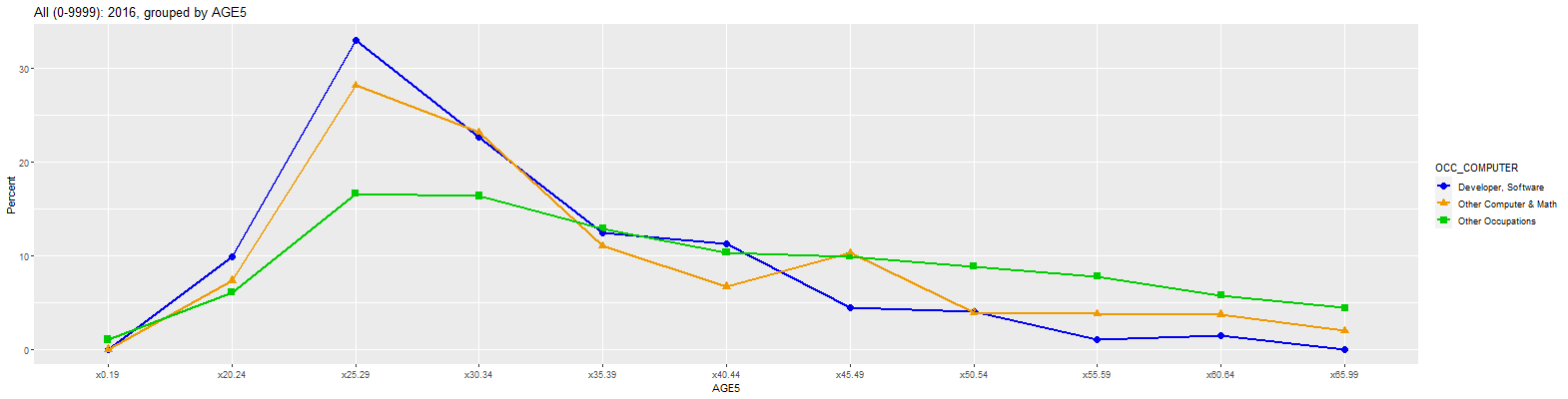
Occupations                           County   count  0-19  20-24  25-29  30-34  35-39  40-44  45-49  50-54  55-59  60-64  65-99
Software Developers        San Francisco, CA   20299   0.0    9.8   32.9   22.6   12.5   11.2    4.5    4.0    1.0    1.4    0.0
Computer and Mathematical  San Francisco, CA   41313   0.0    8.1   29.1   22.9   12.6    9.4    8.5    4.0    2.3    2.3    0.8
All Occupations            San Francisco, CA  508699   1.0    6.3   17.7   16.8   12.8   10.2    9.7    8.5    7.4    5.5    4.2
In order to reproduce some of the numbers for San Francisco, do the following from the initial page:
All (0-9999): 2016, grouped by AGE5 (percent)

  Year          OCC_COMPUTER   Count x0.19 x20.24 x25.29 x30.34 x35.39 x40.44 x45.49 x50.54 x55.59 x60.64 x65.99
1 2016   Developer, Software  20,299   0.0    9.8   32.9   22.6   12.5   11.2    4.5    4.0    1.0    1.4    0.0
2 2016 Other Computer & Math  17,311   0.0    7.3   28.1   23.1   11.0    6.7   10.3    3.9    3.8    3.7    2.0
3 2016     Other Occupations 471,089   1.0    6.1   16.6   16.4   12.9   10.3    9.9    8.8    7.8    5.8    4.4

URL parameters (short)=
?minyear=2016&maxyear=2016&COUNTY=San%20Francisco&geo=COUNTY&occ=All%20(0-9999)&group=AGE5&sortn=0&geomtype=Line%20Graph
As can be seen, the top row for Software Developers in identical but the next two rows are different. This is chiefly because the categories on this page overlap while those above do not overlap. For example, the first is displaying "All Occupations" while the second is displaying "Other Occupations". If you add together the Counts of 20299, 17311, and 471089 above, you do get the count of 508699 given for "All Occupations" on the page.
However, the 20299 and 17311 for Developer and Other Computer & Math in the table above do not add up to the 41313 shown on this page. It is 3703 short. However, a careful examination of that page shows that its "Computer and Mathematical" numbers include OCC values of 110. This code page shows that those include "Computer and information systems managers". This number can be seen via the following steps:
  Year      OCC_COMPUTER Count x20.24 x25.29 x30.34 x35.39 x40.44 x45.49 x50.54 x55.59
1 2016 Other Occupations 3,703    2.3   12.9   23.4   20.9   12.3   22.2    4.0    2.1
This shows that OCC of 110 includes the 3703 missing number shown above. Note that the last step of setting "Minimum Count" to 1 is critical. If left at the default value of 5000, the 3703 value will not be displayed. In fact, that is probably a good reason for leaving "Minimum Count" set to 1 and setting it higher only when desired. The default value may be set to 1, or at least set lower, in the future.
In any case, removing the value in the "Range field1" (and/or setting "Minimum range1" and "Maximum range1" to 0 and 9999) will return to the the original table above. Clicking on the Plot tab will then display a line graph with occupation types along the x-axis and age categories in the legend. To reproduce the first graph in the original story, do the following steps:
As can be seen, this is close to reproducing the first graph in the original story. The blue line for software developer should be identical and the other two lines should be slightly lower since they do not include the prior categories as previously explained. In any event, other available colors can be found at this page and other available palettes can be found at the bottom of this page.
The above numbers can be updated to 2021 by clicking on the Output tab and changing "First Year" and "Last Year" to 2021. That will display the following table:
Computer Occupations, Employment by Age, San Francisco County: 2021
2021  Total count = 157,815,522

AMERICAN COMMUNITIES SURVEY: 2021
(STATE=CA, COUNTY=San Francisco)

All (0-9999): 2021, grouped by AGE5 (percent)

  Year          OCC_COMPUTER   Count x0.19 x20.24 x25.29 x30.34 x35.39 x40.44 x45.49 x50.54 x55.59 x60.64 x65.99
1 2021   Developer, Software  29,638   0.0    9.5   27.4   26.8   12.1    9.6    8.5    2.3    2.6    0.6    0.6
2 2021 Other Computer & Math  21,799   0.3   10.4   21.6   21.3   13.1   11.7    6.9    5.5    4.2    3.2    1.8
3 2021     Other Occupations 400,485   1.4    5.5   12.5   15.9   12.6   11.5    9.4    9.8    8.3    6.9    6.2

URL parameters (short)=
?minyear=2021&maxyear=2021&COUNTY=San%20Francisco&geo=COUNTY&occ=All%20(0-9999)&group=AGE5&sortn=0&mincount=1&color=Set1&geomtype=Line%20Graph
Clicking on the Plot tab will display the following line graph:

A careful comparison of the 2016 and 2021 numbers show that the numbers appear to skew slightly older from 2016 to 2021. It's possible to compare them to all occupations by going back to the Output tab and changing "Row var" to OCC. That will display the following table:
All Occupations, Employment by Age, San Francisco County: 2021
2021  Total count = 157,815,522

AMERICAN COMMUNITIES SURVEY: 2021
(STATE=CA, COUNTY=San Francisco)

All (0-9999): 2021, grouped by AGE5 (percent)

   Year      OCC   Count x0.19 x20.24 x25.29 x30.34 x35.39 x40.44 x45.49 x50.54 x55.59 x60.64 x65.99
1  2021  Manager  76,242   0.0    3.3   13.2   19.1   16.4   14.3   10.1    8.6    4.8    5.2    5.0
2  2021 Business  30,558   0.0    4.3   17.8   19.2   12.3   10.9    6.3   10.2    6.4    7.4    5.1
3  2021  Finance  14,861   0.0    7.0   17.2   17.9    9.1    9.3   17.6    7.4    7.7    4.9    1.9
4  2021 CompMath  51,437   0.1    9.9   24.9   24.5   12.5   10.5    7.8    3.6    3.3    1.7    1.1
5  2021 Engineer  13,239   0.0    8.1   24.8   18.2   14.3   13.9    4.8    1.5    7.0    3.0    4.4
6  2021  LifeSci  16,699   0.0    4.3   12.5   30.2    6.8   15.8    7.8   12.3    4.1    4.5    1.6
7  2021  SocServ   5,996   0.6    0.8   24.6   14.9    6.5    6.0    7.3    3.6   20.4    5.5    9.8
8  2021    Legal  14,989   0.0    0.6   11.1   16.1   22.2   10.9   11.5    8.7    7.2    4.4    7.4
9  2021     Educ  25,568   1.2    4.4   14.4   11.8   12.8   12.4    9.6   10.8   11.4    4.4    6.9
10 2021     Arts  22,715   0.0    9.2   12.3   17.9   20.1    9.4    4.6    9.0    5.3    4.4    7.8
11 2021 HlthDiag  23,495   0.0    0.1    7.8   20.1   16.0   10.5   14.4    8.0    8.6    8.0    6.4
12 2021 HlthCare  11,502   0.0    6.1    8.5    5.9    6.3    6.5    8.1   13.3   11.2   15.5   18.6
13 2021    Other 144,621   3.7    7.8    9.8   12.0    9.6   10.8    9.3   11.3   10.4    8.8    6.5

URL parameters (short)=
?minyear=2021&maxyear=2021&COUNTY=San%20Francisco&geo=COUNTY&occ=All%20(0-9999)&group=AGE5&sortn=0&mincount=1&color=Set1&geomtype=Line%20Graph
Clicking on the Plot tab and changing "Color" to Set3 (in order to define enough colors) will display a line graph with 12 lines. It makes it a little easier to distinguish the lines from each other by checking the "Use linetype" checkbox, resulting in the following line graph:

As can be seen Computer & Math occupations (CompMath) appear to skew the youngest, followed by Engineering Occupations (Engineer) and Life Science Occupations (LifeSci). Interestingly, Healthcare Support Occupations (HlthCare) are the occupations that seems to skew the oldest, reaching their highest level in the 65 and older age bracket. The occupations with the most balanced distribution of age brackets appears to be Education Occupations (Educ) with the levels trailing off after the 55-59 bracket. It should be noted that Set3 has 12 colors and hence did not have enough for Social Services (SocServ).
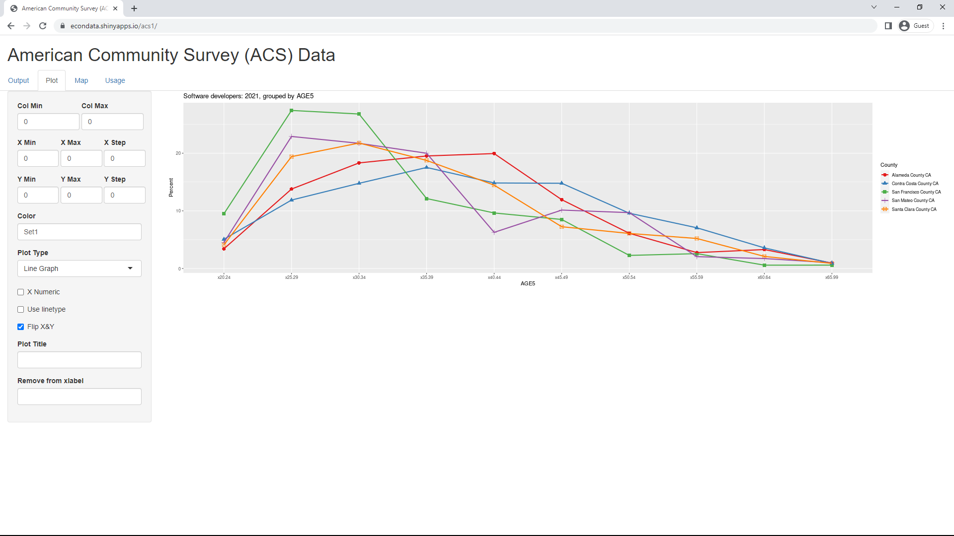
It's possible to compare the age distribution of software developers in San Francisco County to other Bay Area counties by switching back to the Output tab and doing the following:
Software Developers, Employment by Age, San Francisco Bay Area: 2021
2021  Total count = 1,851,196

AMERICAN COMMUNITIES SURVEY: 2021
(STATE=CA, COUNTY=Alameda|Santa Clara|San Francisco|San Mateo|Contra Costa)

Software developers: 2021, grouped by AGE5 (percent)

  Year                  COUNTY  Count x20.24 x25.29 x30.34 x35.39 x40.44 x45.49 x50.54 x55.59 x60.64 x65.99
1 2021   Santa Clara County CA 90,311    4.1   19.4   21.8   18.7   14.5    7.2    6.1    5.2    2.1    0.9
2 2021       Alameda County CA 50,566    3.4   13.8   18.3   19.5   19.9   11.9    6.1    2.8    3.3    0.9
3 2021 San Francisco County CA 29,638    9.5   27.4   26.8   12.1    9.6    8.5    2.3    2.6    0.6    0.6
4 2021     San Mateo County CA 18,130    4.5   22.9   21.7   20.0    6.3   10.1    9.7    2.1    1.7    1.0
5 2021  Contra Costa County CA 11,269    5.1   11.9   14.8   17.5   14.8   14.8    9.6    7.1    3.6    0.9

URL parameters (short)=
?minyear=2021&maxyear=2021&COUNTY=Alameda|Santa%20Clara|San%20Francisco|San%20Mateo|Contra%20Costa&geo=COUNTY&occ=Software%20developers&group=AGE5&color=Set1&geomtype=Line%20Graph
It was previously noted that the 2016 and 2021 numbers show that the numbers appear to skew slightly older from 2016 to 2021. It's possible to look at the change for every year from 2016 to 2021 by doing the following:
Software Developers, Employment by Age, San Francisco County: 2016-2021
2021  Total count = 1,851,196
2020  Total count = 1,790,632
2019  Total count = 905,923
2018  Total count = 1,350,240
2017  Total count = 1,372,973
2016  Total count = 1,276,877

AMERICAN COMMUNITIES SURVEY: 2016-2021
(STATE=CA, COUNTY=San Francisco)

Software developers: 2016-2021, grouped by AGE5, STATE=CA, COUNTY=San Francisco (percent)

  Year                  COUNTY  Count x20.24 x25.29 x30.34 x35.39 x40.44 x45.49 x50.54 x55.59 x60.64 x65.99 x0.19
1 2016 San Francisco County CA 20,299    9.8   32.9   22.6   12.5   11.2    4.5    4.0    1.0    1.4     NA    NA
2 2017 San Francisco County CA 22,428   10.4   23.8   30.8   17.9    9.5    2.3    3.3    1.5    0.5     NA    NA
3 2018 San Francisco County CA 26,493   11.7   29.2   28.4   15.3    8.7    3.6    1.3    1.0    0.2    0.6    NA
4 2019 San Francisco County CA 32,358    7.2   35.8   26.8   10.4    8.7    3.5    3.6    1.8    2.0    0.2    NA
5 2020 San Francisco County CA 32,535    9.6   31.7   32.9   10.9    4.3    3.7    2.5    2.4    1.2    0.6   0.3
6 2021 San Francisco County CA 29,638    9.5   27.4   26.8   12.1    9.6    8.5    2.3    2.6    0.6    0.6    NA

URL parameters (short)=
?minyear=2016&maxyear=2021&COUNTY=San%20Francisco&geo=COUNTY&occ=Software%20developers&group=AGE5&mincount=1&color=Set1&geomtype=Line%20Graph
Clicking on the Plot tab will then display the following line graph:
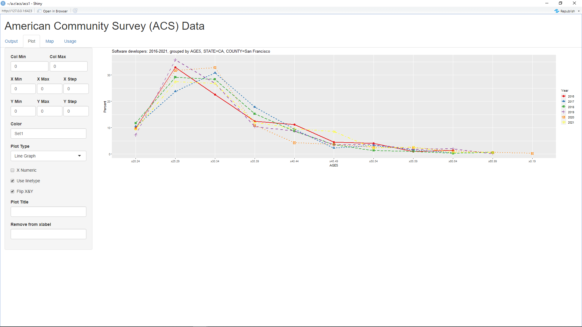
As can be seen, the ages were highly skewed to the 25-29 bracket in 2016 but became much less so in 2017. However, it then became more skewed toward that bracket in 2018 and reached a maximum in 2019. At the same time, 2017 through 2019 became less skewed toward the 30-34 and 34-39 brackets. However, these trends again reversed and began to move in the other direction in 2020 and 2021. As noted on this page, the ACS 2020 data "uses experimental weights to correct for the effects of the COVID-19 pandemic on the 2020 ACS data collection".