
On December 26, 2016, economist George Borjas posted an article on his blog titled Where Did 2.5 Million Native Working Men Go?. It includes a graph showing a substantial rise in the number of prime-age native men who do not work at all during an entire calendar year. It also includes the simple Stata code which was used to generate the graph using CPS (Consumer Population Survey) data. Stata is a statistical language widely used in academia. The following describes how to replicate the data and graph in the statistical language R, another widely used statistical language which has the advantage of being freely available under the GNU General Public License.
Following are instructions for extracting the required data from IPUMS, the Integrated Public Use Microdata Series:
Variable   Variable Label                              Type   16  15  14  13  12  11  10  09  08  07  06  05  04  03  02  01  00  99  98  97  96  95  94
---------  ------------------------------------------  ----  --- --- --- --- --- --- --- --- --- --- --- --- --- --- --- --- --- --- --- --- --- --- ---
YEAR       Survey year [preselected]                     H     X   X   X   X   X   X   X   X   X   X   X   X   X   X   X   X   X   X   X   X   X   X   X
SERIAL     Household serial number [preselected]         H     X   X   X   X   X   X   X   X   X   X   X   X   X   X   X   X   X   X   X   X   X   X   X
HWTSUPP    Household weight, Supplement [preselected]    H     X   X   X   X   X   X   X   X   X   X   X   X   X   X   X   X   X   X   X   X   X   X   X
CPSID      CPSID, household record [preselected]         H     .   .   .   .   .   .   X   X   X   X   X   X   X   X   X   X   X   X   X   X   X   X   X
ASECFLAG   Flag for ASEC [preselected]                   H     X   X   X   X   X   X   X   X   X   X   X   X   X   X   X   X   X   X   X   X   X   X   X
HFLAG      Flag for the 3/8 file 2014 [preselected]      H     .   .   X   .   .   .   .   .   .   .   .   .   .   .   .   .   .   .   .   .   .   .   .
MONTH      Month [preselected]                           H     X   X   X   X   X   X   X   X   X   X   X   X   X   X   X   X   X   X   X   X   X   X   X
PERNUM     Person number in sample unit [preselected]    P     X   X   X   X   X   X   X   X   X   X   X   X   X   X   X   X   X   X   X   X   X   X   X
CPSIDP     CPSID, person record [preselected]            P     .   .   .   .   .   .   X   X   X   X   X   X   X   X   X   X   X   X   X   X   X   X   X
WTSUPP     Supplement Weight [preselected]               P     X   X   X   X   X   X   X   X   X   X   X   X   X   X   X   X   X   X   X   X   X   X   X
STATEFIP   State (FIPS code)                             H     X   X   X   X   X   X   X   X   X   X   X   X   X   X   X   X   X   X   X   X   X   X   X
METFIPS    Metropolitan area FIPS code                   H     X   X   X   X   X   X   X   X   X   X   X   X   X   X   X   X   X   X   X   X   X   X   X
AGE        Age                                           P     X   X   X   X   X   X   X   X   X   X   X   X   X   X   X   X   X   X   X   X   X   X   X
SEX        Sex                                           P     X   X   X   X   X   X   X   X   X   X   X   X   X   X   X   X   X   X   X   X   X   X   X
CITIZEN    Citizenship status                            P     X   X   X   X   X   X   X   X   X   X   X   X   X   X   X   X   X   X   X   X   X   X   X
EDUC       Educational attainment recode                 P     X   X   X   X   X   X   X   X   X   X   X   X   X   X   X   X   X   X   X   X   X   X   X
EMPSTAT    Employment status                             P     X   X   X   X   X   X   X   X   X   X   X   X   X   X   X   X   X   X   X   X   X   X   X
WKSWORK1   Weeks worked last year                        P     X   X   X   X   X   X   X   X   X   X   X   X   X   X   X   X   X   X   X   X   X   X   X
UHRSWORKLY Usual hours worked per week (last yr)         P     X   X   X   X   X   X   X   X   X   X   X   X   X   X   X   X   X   X   X   X   X   X   X
> source("nowork1ed.R")
[1] "***** USING current cc dataframe. If error, enter 'rm(cc)' and rerun. *****"
[1] "4268777  Initial number of records"
[1] "4268777  1994 to present"
[1] "4268777  the United States"
[1] "1798834  AGE 25 to 54"
[1] "861800  MEN"
[1] "861800  SUPPLEMENT WEIGHT >= 0"
   YEAR IMMIGRANT NATIVE
1  1994     11.07   8.20
2  1995     10.37   7.92
3  1996      9.71   8.16
4  1997      9.37   7.71
5  1998      8.14   7.48
6  1999      7.84   7.82
7  2000      7.47   7.64
8  2001      8.11   7.74
9  2002      8.00   8.58
10 2003      9.10   9.23
11 2004      9.30  10.36
12 2005      8.33  10.40
13 2006      7.73  10.08
14 2007      7.69   9.89
15 2008      8.14  10.35
16 2009      8.03  11.26
17 2010     10.68  13.11
18 2011     11.27  14.40
19 2012     10.50  14.69
20 2013      9.76  14.04
21 2014      8.53  14.30
22 2015      9.76  13.72
23 2016      9.33  12.99
Press enter to continue, escape to exit
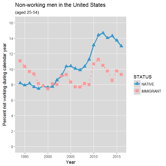
Below is George Borjas' graph from his post, followed by the first graph generated by the program. As can be seen, the program does appear to replicate the numbers in Borjas' graph exactly. Also, the graphs show an interesting pattern. For native men, the percentage not working for the entire year was about 8 percent from 1994 to 2001. Then, following the collapse of the tech bubble, the percentage increased to about 10 percent in 2004 to 2007. Then, following the financial crisis, the percentage skyrocketed to nearly 15 pecent in 2012 but has since fallen back to about 13 percent.
The percentages for immigrant men have been somewhat more steady. They fell from about 11 percent in 1994 to about 8 percent in 1998 and continued there through 2002. They did rise briefly to about 9 percent in 2003 and 2004 but fell back to about 8 percent from 2005 through 2009. Following the financial crisis, they rose to over 11 percent in 2011 but have fallen back to about 9 percent since then.
The rest of the program divides this group of men aged 25-54 into 6 groups according to their educations, specifically the highest degree that they received. The six groups are as follows:
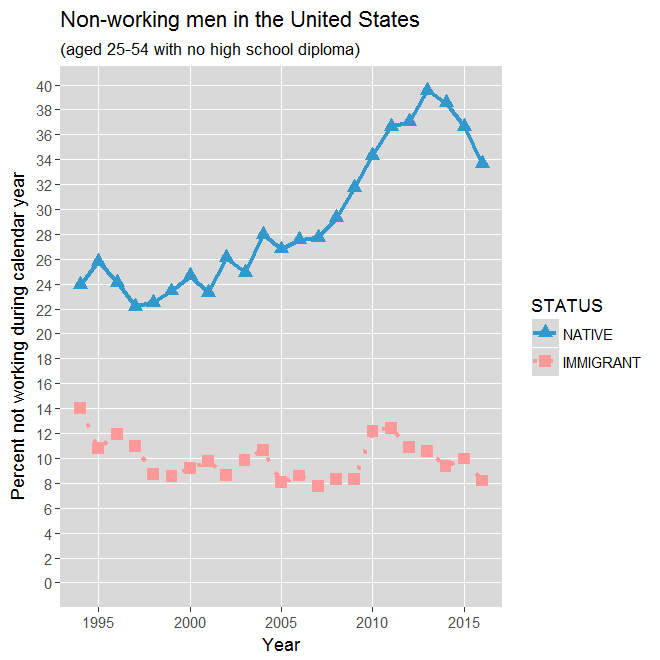
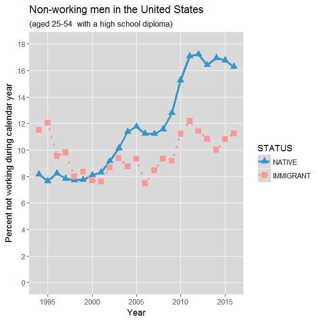
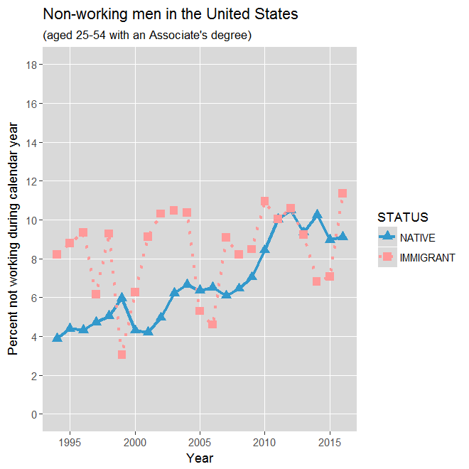
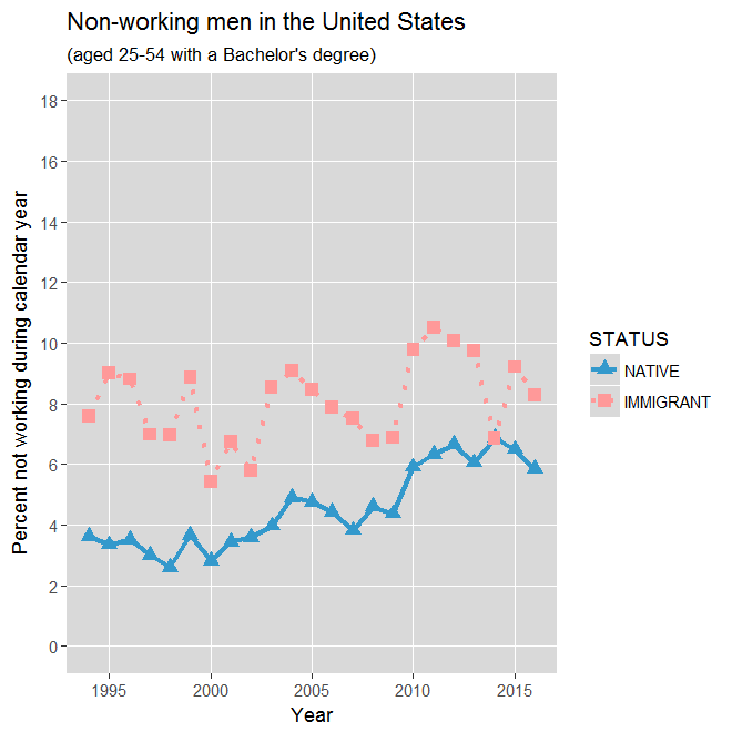
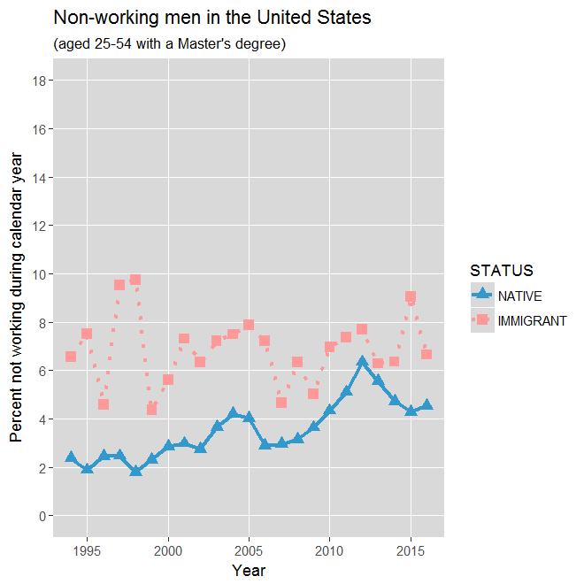
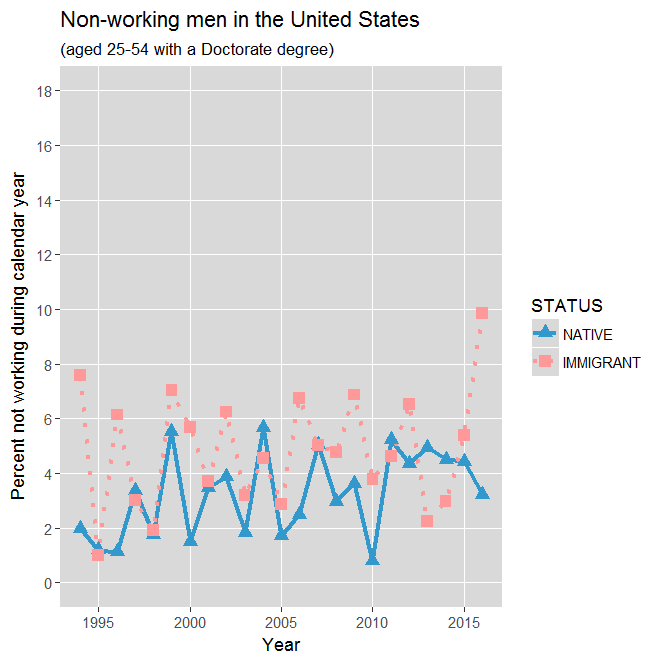
As can be seen from the first graph, the percentages of non-working men is much higher for natives than for immigrants when looking at those without a high school diploma. The second graph shows that the percentages have likewise been somewhat larger since abut 2004 for those with just a high school diploma. For Associate's degrees, the percentages are similiar and for bachelor, master, and doctorate degrees, the percentages for natives is actually a bit lower than for immigrants. Also, most of the native subgroups seem to follow a pattern very similar to the entire native group except at different levels. There is a pre-tech-crash level that goes from 1994 to 2001, a post-tech-crash level that goes from about 2004 to 2007 or 2008, a post-financial crisis peak that is reached in 2012 or 2013, and then a current recovery low reached in 2016. This can be better seen in the first of the following two graphs which shows the percentages for all of the native subgroups in one graph:
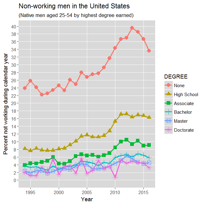
As can be seen, the percentages are by far the highest for native men without a high school diploma and generally get lower and lower with each higher level of degree. Interestingly, this is much less the case for immigrant men, shown in the last graph above. Some of this may be due to the greater volatility of the percentages, likely due to the smaller sample sizes for immigrants. Still, their percentages range only up to about 14 percent whereas the native percentages range up to about 40 percent. Again, this difference is mainly due to high percentages for native men without a high school diploma and, since about 2004, native men with a high school diploma.
Someone suggested to me that many of the prime-age men who are not working may be on disability. To check this, I looked at the variable EMPSTAT whose codes are given at this link. As can be seen, this variable indicates those persons who are not in the labor force for the three reasons of 1) unable to work, 2) retired, and 3) other. The R program at http://econdataus.com/nowork1ed.R was modified to filter out men who were unable to work or retired, creating the program at http://econdataus.com/nowork1edaw.R. These categories are in the CPS data only from 1995 on so the year 1994 was also dropped from the data. Following is the start of the resulting output from if this new program is placed in the same directory as cps16.csv and run:
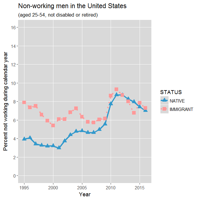
Below is the first graph which replicates George Borjas' graph, followed by the first graph generated by this modified program. As can be seen, omitting men who are unable to work or are retired greatly lowers the percentage of non-working prime-age men. In addition, it changes the relationship between non-working native and immigrant men. When such groups are included, the percentages of non-working native men has been greater than non-working immigrants since 2004. When they are excluded, however, the percentages of non-working native men are lower than for non-working immigrants through 2009 and have been fairly close to the same since then.
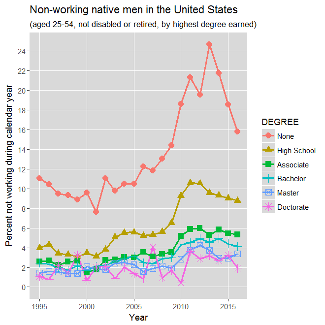
The following graphs show the percentages for all of the native subgroups using the old and new programs.
The tables that correspond to these two graphs are below. As can be seen, the percentages of non-working native men are less when disabled and retired men are excluded. However, the percentages still follow similar patterns. There is a pre-tech-crash level that goes from 1994 to 2001, a post-tech-crash level that goes from about 2004 to 2007 or 2008, a post-financial crisis peak that is reached in 2012 or 2013, and then a current recovery low reached in 2016. Also, the percentages are by far the highest for native men without a high school diploma and generally get lower and lower with each higher level of degree.
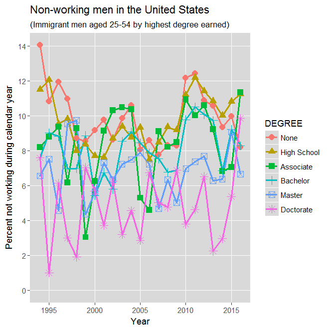
The tables that correspond to these two graphs are below. As can be seen, any changes following the tech-crash or financial crisis are less discernible for immigrants. The overall levels seem slightly lower when disabled and retired men are excluded, topping out in 2011 at just above 10 rather than 12 percent. Likewise, the percentages tend to be lower for immigrant men with each higher level of degree but this is likewise less discernible.
A Look At Non-working Prime-age Men Who Are Not Disabled or Retired
> source("nowork1edaw.R")
[1] "READING cps16.csv"
[1] "4268777  Initial number of records"
[1] "4117834  1995 to present"
[1] "4117834  the United States"
[1] "1734411  AGE 25 to 54"
[1] "830818  MEN"
[1] "830818  SUPPLEMENT WEIGHT >= 0"
[1] "824713  NOT RETIRED"
[1] "790226  ABLE TO WORK"
   YEAR IMMIGRANT NATIVE
1  1995      7.90   3.94
2  1996      7.37   4.09
3  1997      7.53   3.43
4  1998      6.57   3.28
5  1999      5.93   3.20
6  2000      5.41   3.21
7  2001      6.11   2.99
8  2002      6.08   3.74
9  2003      6.83   4.41
10 2004      7.25   4.77
11 2005      6.34   4.84
12 2006      5.79   4.66
13 2007      5.72   4.64
14 2008      6.05   4.98
15 2009      6.17   5.57
16 2010      8.62   7.75
17 2011      9.30   8.72
18 2012      8.70   8.70
19 2013      8.02   8.28
20 2014      6.77   7.96
21 2015      7.84   7.42
22 2016      7.30   7.02
Press enter to continue, escape to exit
The output above suggests that there are many more prime-age men who are unable to work than are retired. It shows that there are 34,487 (824,713 - 790,226) records for prime-age men who are unable to work but only 6,105 (830,818 - 824,713) records for prime-age men who are retired.
[1] "Non-working men in the United States"                          |  [1] "Non-working native men in the United States"
[1] "(Native men aged 25-54, by highest degree earned)"             |  [1] "(aged 25-54, not disabled or retired, by highest degree earned)"
[1] ""                                                              |  [1] ""
   year     None High School Associate Bachelor   Master Doctorate  |     year      None High School Associate Bachelor   Master Doctorate
1  1994 23.93476    8.158448  3.896971 3.640087 2.369354 1.9878545  |
2  1995 25.79986    7.659562  4.388986 3.348897 1.890308 1.1966235  |  1  1995 11.048307    3.969391  2.591929 2.442985 1.436833 1.0644856
3  1996 24.09733    8.246367  4.332988 3.522857 2.458127 1.1240355  |  2  1996 10.431690    4.329267  2.700989 2.311037 1.558790 0.7813831
4  1997 22.17640    7.834706  4.719395 3.003711 2.475704 3.3732589  |  3  1997  9.500403    3.396144  2.232627 1.985542 1.500015 2.1844244
5  1998 22.50329    7.733667  5.044659 2.598489 1.794520 1.7700976  |  4  1998  9.326256    3.307981  2.557800 1.714335 1.358966 1.4345468
6  1999 23.42595    7.751093  5.971421 3.677120 2.320554 5.5305467  |  5  1999  8.912069    3.072446  2.651000 2.165487 1.379175 3.2346097
7  2000 24.64538    8.107736  4.301428 2.826800 2.856068 1.5169964  |  6  2000  9.598931    3.447551  1.519486 1.653959 2.091263 0.6489769
8  2001 23.33722    8.302969  4.219798 3.444472 2.983891 3.4924304  |  7  2001  7.640450    3.103152  1.774484 2.114655 1.845905 2.0178369
9  2002 26.10195    9.170032  4.961840 3.600853 2.761848 3.8744776  |  8  2002 11.031562    3.827119  2.713626 2.213669 1.753767 2.0599418
10 2003 24.90467   10.135294  6.224749 3.974275 3.665574 1.8380122  |  9  2003  9.788979    5.053351  2.779903 2.561775 2.420605 0.8798000
11 2004 27.98283   11.385504  6.673425 4.913583 4.202391 5.6700937  |  10 2004 10.492163    5.520809  3.034578 2.895233 2.500184 2.0146012
12 2005 26.80580   11.764377  6.361591 4.756703 4.028958 1.7104130  |  11 2005 10.508144    5.561023  3.005369 3.118164 2.270327 1.3519057
13 2006 27.53624   11.223668  6.524083 4.435543 2.895372 2.4916975  |  12 2006 12.228161    5.237080  3.550063 2.469026 1.586251 0.8196643
14 2007 27.75558   11.214378  6.097780 3.827268 2.960263 5.0618161  |  13 2007 11.827666    5.319175  3.099831 2.381781 1.892904 4.0588827
15 2008 29.30280   11.571590  6.461713 4.605218 3.157504 2.9787060  |  14 2008 13.041878    5.603615  3.355218 2.878247 2.146078 0.9251455
16 2009 31.72768   12.788053  7.043775 4.379115 3.644760 3.6361968  |  15 2009 14.408642    6.527108  3.514557 2.986322 1.926392 1.7155335
17 2010 34.31836   15.274047  8.440003 5.912770 4.336778 0.7922547  |  16 2010 18.588905    9.290675  5.170669 4.289186 2.838599 0.4186806
18 2011 36.63066   17.091594 10.024771 6.340361 5.108762 5.2275024  |  17 2011 21.305855   10.570562  5.892957 4.527796 3.757421 3.6489758
19 2012 37.02843   17.216450 10.482695 6.649542 6.350413 4.3658314  |  18 2012 19.545043   10.556135  5.979951 4.920452 4.254250 2.8845053
20 2013 39.52832   16.409264  9.349281 6.062037 5.551721 4.9366017  |  19 2013 24.655405    9.570819  5.281138 4.509749 3.731786 3.1907374
21 2014 38.55372   16.939782 10.255942 6.869011 4.722501 4.5033449  |  20 2014 21.790390    9.314117  5.831258 4.948481 2.925943 2.6825799
22 2015 36.66128   16.758037  8.971155 6.500578 4.278258 4.4359567  |  21 2015 18.560155    9.043120  5.460408 4.398864 2.909817 3.2347204
23 2016 33.64799   16.273820  9.122731 5.846723 4.537243 3.2254183  |  22 2016 15.781907    8.780200  5.316584 4.116720 3.387643 1.9143537
Press enter to continue, escape to exit                                Press enter to continue, escape to exit
The following graphs show the percentages for all of the immigrant subgroups using the old and new programs.
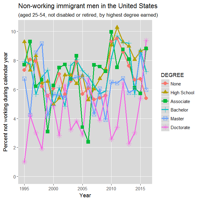
[1] "Non-working men in the United States"                            |  [1] "Non-working immigrant men in the United States"
[1] "(Immigrant men aged 25-54, by highest degree earned)"            |  [1] "(aged 25-54, not disabled or retired, by highest degree earned)"
[1] ""                                                                |  [1] ""
   year      None High School Associate  Bachelor   Master Doctorate  |     year     None High School Associate Bachelor   Master Doctorate
1  1994 14.033034   11.493449  8.201668  7.587995 6.557907  7.584898  |
2  1995 10.820140   12.052305  8.789175  9.027794 7.523659  1.013484  |  1  1995 7.330412    9.267499  7.693659 7.927455 6.733559  1.013484
3  1996 11.932034    9.526647  9.359483  8.814626 4.581276  6.144976  |  2  1996 8.059229    7.321660  9.287818 7.743603 4.249432  4.223218
4  1997 10.956381    9.813705  6.174171  6.984775 9.539714  3.012604  |  3  1997 7.925817    8.307901  6.209094 5.661433 8.527706  3.012604
5  1998  8.714946    7.996812  9.291066  6.974422 9.747802  1.910817  |  4  1998 6.206645    6.445191  6.650490 6.852248 9.166293  1.910817
6  1999  8.531789    8.363127  3.048060  8.867331 4.361156  7.036046  |  5  1999 5.547831    6.545960  3.087448 7.322615 4.161811  5.581273
7  2000  9.169114    7.697235  6.262186  5.433323 5.624510  5.677590  |  6  2000 6.053492    4.959868  6.262186 4.894527 5.683816  4.834512
8  2001  9.758264    7.620222  9.136511  6.750867 7.315921  3.721288  |  7  2001 7.064123    5.393381  7.485772 6.117435 5.603652  2.814083
9  2002  8.617679    8.694351 10.315303  5.793964 6.351902  6.252799  |  8  2002 5.663988    6.987875  7.710801 4.840935 5.455150  6.313112
10 2003  9.840201    9.392804 10.470152  8.537524 7.234353  3.209059  |  9  2003 6.565908    6.976276  6.715102 7.666644 6.711454  3.209059
11 2004 10.604418    8.756340 10.372942  9.079274 7.497957  4.564734  |  10 2004 7.900639    6.390199  8.296535 8.037116 6.839079  3.820686
12 2005  8.064483    9.326450  5.301334  8.456405 7.884339  2.868461  |  11 2005 5.687213    6.949563  3.397037 7.274183 6.914273  2.868461
13 2006  8.590182    7.471582  4.605281  7.873194 7.227543  6.732683  |  12 2006 6.074488    5.273809  2.378777 6.913610 6.270162  6.732683
14 2007  7.757602    8.479059  9.103436  7.529590 4.676437  5.026372  |  13 2007 5.310396    6.026410  7.685323 6.271134 4.276588  5.026372
15 2008  8.312823    9.350206  8.213938  6.774803 6.344314  4.767132  |  14 2008 5.408784    6.726654  7.565692 5.693464 6.053311  3.874791
16 2009  8.276154    9.178335  8.483715  6.876599 5.042763  6.877191  |  15 2009 5.564011    7.375030  7.233666 5.889929 3.897021  5.550368
17 2010 12.175131   11.198450 10.943474  9.779326 6.959284  3.792619  |  16 2010 9.293035    9.037258  9.945069 8.138775 6.512681  2.562861
18 2011 12.420359   12.193465 10.033817 10.500795 7.358617  4.638000  |  17 2011 9.504431   10.255605  7.508032 9.686682 6.434427  3.376363
19 2012 10.866810   11.412889 10.593446 10.068147 7.693326  6.525689  |  18 2012 8.566408    9.258888  8.750570 9.214269 6.767762  6.442759
20 2013 10.560259   10.835212  9.226796  9.736871 6.290508  2.255934  |  19 2013 7.618328    8.959526  8.066934 9.174862 5.754231  2.255934
21 2014  9.348807   10.006865  6.818387  6.860362 6.360493  2.969372  |  20 2014 6.665344    8.048224  6.094223 5.654849 6.006511  3.014964
22 2015  9.956958   10.806339  7.066466  9.217391 9.067074  5.380317  |  21 2015 6.727441    8.639447  5.722436 8.697853 8.430892  5.380317
23 2016  8.188258   11.252606 11.346355  8.282496 6.654622  9.846073  |  22 2016 5.388443    8.808517  8.803258 7.224750 5.967010  9.367113
Press enter to continue, escape to exit                                  Press enter to continue, escape to exit
In summary, the 2.5 million number in George Borjas' question of "Where Did 2.5 Million Native Working Men Go?" is based on a rise of 5 percent, from 8 percent to 13 percent, in a population of about 50 million prime-age native men. Excluding those men who are unable to work (presumedly on disability) or retired causes the rise to be 3 percent, from 4 to 7 percent. Three percent of 50 million is 1.5 million. Hence, it would seem that about a million of the 2.5 million prime-age native men became disabled or retired (chiefly the former) and the other 1.5 million includes the unemployed and those who disappeared from the labor force with the reason of "other". I would presume that this latter group is chiefly men who were unable to find work but dropped off the unemployment rolls, having used up all of their allowed unemployment.
A Look At Non-working Prime-age Men Using R: 1994-2018
A Look At Mariel Using R