On April 4, 2016, economist George Borjas posted an article on his blog titled An Empirical Exercise: Mariel. It includes a graph showing the negative effect of the Marielitos who came to Miami via the Mariel boatlift in 1980. It also includes a video that explains how the graph was created using CPS (Consumer Population Survey) data and Stata, a statistical language widely used in academia. The following describes how to replicate the data and graph in the statistical language R, another widely used statistical language which has the advantage of being freely available under the GNU General Public License.
Following are instructions for extracting the required data from IPUMS, the Integrated Public Use Microdata Series:
Variable  Variable Label                              Type   91   90   89   88   87   86   85   84   83   82   81   80   79   78   77   76
--------  ------------------------------------------  ----  ---- ---- ---- ---- ---- ---- ---- ---- ---- ---- ---- ---- ---- ---- ---- ----
YEAR      Survey year [preselected]                     H     X    X    X    X    X    X    X    X    X    X    X    X    X    X    X    X
SERIAL    Household serial number [preselected]         H     X    X    X    X    X    X    X    X    X    X    X    X    X    X    X    X
HWTSUPP   Household weight, Supplement [preselected]    H     X    X    X    X    X    X    X    X    X    X    X    X    X    X    X    X
ASECFLAG  Flag for ASEC [preselected]                   H     X    X    X    X    X    X    X    X    X    X    X    X    X    X    X    X
MONTH     Month [preselected]                           H     X    X    X    X    X    X    X    X    X    X    X    X    X    X    X    X
PERNUM    Person number in sample unit [preselected]    P     X    X    X    X    X    X    X    X    X    X    X    X    X    X    X    X
WTSUPP    Supplement Weight [preselected]               P     X    X    X    X    X    X    X    X    X    X    X    X    X    X    X    X
METAREA   Metropolitan area                             H     X    X    X    X    X    X    X    X    X    X    X    X    X    X    X    X
AGE       Age                                           P     X    X    X    X    X    X    X    X    X    X    X    X    X    X    X    X
SEX       Sex                                           P     X    X    X    X    X    X    X    X    X    X    X    X    X    X    X    X
HISPAN    Hispanic origin                               P     X    X    X    X    X    X    X    X    X    X    X    X    X    X    X    X
EDUC      Educational attainment recode                 P     X    X    X    X    X    X    X    X    X    X    X    X    X    X    X    X
WKSWORK1  Weeks worked last year                        P     X    X    X    X    X    X    X    X    X    X    X    X    X    X    X    X
INCWAGE   Wage and salary income                        P     X    X    X    X    X    X    X    X    X    X    X    X    X    X    X    X
> source("mariel1.R")
[1] "READ mariel1.csv"
[1] "FILTER DATA"
[1] "OUTPUT SAMPLE COUNTS OF DATA"
   YEAR NON_MIAMI MIAMI MIAMI3
1  1975      4660    17     NA
2  1976      5425    24     67
3  1977      4972    26     72
4  1978      4515    22     65
5  1979      5135    17     57
6  1980      4895    18     56
7  1981      4213    21     68
8  1982      3982    29     68
9  1983      3665    18     63
10 1984      3529    16     51
11 1985      3374    17     50
12 1986      3255    17     52
13 1987      3239    18     52
14 1988      2874    17     53
15 1989      2903    18     40
16 1990      2798     5     NA
The above table shows the sample counts for the data. As can be seen in the second to the rightmost column, the sample counts for Miami workers range from 5 in 1990 to 29 in 1982. To remedy these relatively small sample sizes, the analysis looks at the 3-year moving average. As can be seen in the rightmost column, this increases the sample counts for Miami workers such that they range from 40 in 1988-1990 to 72 in 1976-1978. The output continues:
[1] "OUTPUT DATA MATCHING THAT SHOWN AT 6:40 IN VIDEO AT"
[1] "  https://gborjas.org/2016/04/04/an-empirical-exercise-mariel/"
   YEAR NON_MIAMI    MIAMI
1  1975  321.4743 276.5552
2  1976  330.4234 301.0069
3  1977  328.6451 345.3347
4  1978  329.5881 285.8485
5  1979  322.3343 285.5436
6  1980  303.8424 284.9430
7  1981  294.0709 232.7979
8  1982  280.6094 202.9967
9  1983  279.8923 214.8615
10 1984  274.0356 217.5500
11 1985  276.8372 159.1372
12 1986  291.6120 154.9670
13 1987  289.1380 213.8362
14 1988  281.1351 207.5364
15 1989  267.0321 278.9775
16 1990  256.9168 245.9369
As noted, these appear to duplicate the numbers shown at 6:40 in the video. These are yearly figures, before the 3-year moving averages are calculated. The output continues:
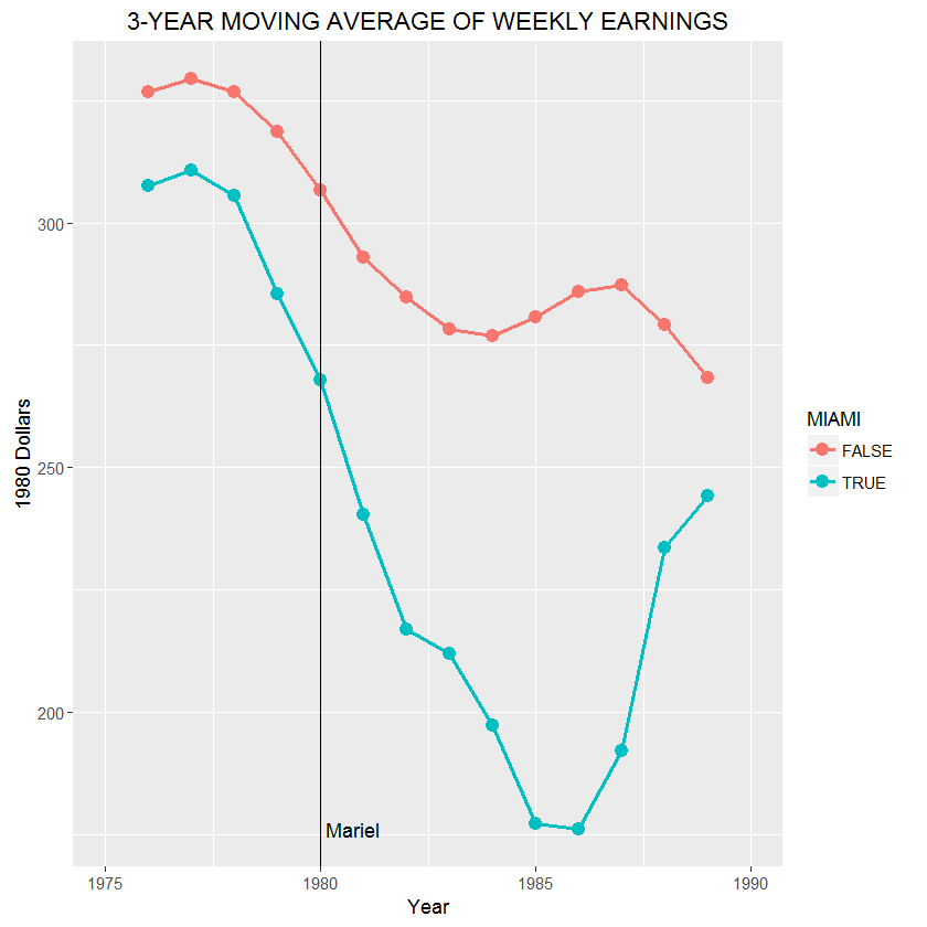
[1] "OUTPUT 3-YEAR MOVING AVERAGE DATA GRAPHED AT 8:20 IN VIDEO"
   YEAR NON_MIAMI    MIAMI
1  1975        NA       NA
2  1976  326.8476 307.6323
3  1977  329.5522 310.7300
4  1978  326.8558 305.5756
5  1979  318.5882 285.4450
6  1980  306.7492 267.7615
7  1981  292.8409 240.2459
8  1982  284.8576 216.8854
9  1983  278.1791 211.8027
10 1984  276.9217 197.1829
11 1985  280.8282 177.2181
12 1986  285.8624 175.9801
13 1987  287.2951 192.1132
14 1988  279.1018 233.4500
15 1989  268.3614 244.1503
16 1990        NA       NA
Warning messages:
1: Removed 4 rows containing missing values (geom_path).
2: Removed 4 rows containing missing values (geom_point).
>
This shows the 3-year moving averages calculated using the average of the year in question plus the prior and following years. The years 1975 and 1990 are undefined because the data for the prior and following years, respectively, are not available. The two warning messages are caused by these undefined values. In any event, the above values are used to create the following graph:
As can be seen, this graph appears to replicate the graph in the original article. The vertical line shows the year when the Mariel boatlift occurred. As can be seen, the gap between the wages of low-skilled native workers in Miami and outside Miami increased sharply until 1985 or 1986 and then recovered through 1989.