UPDATE: See the updated analysis and evaluation by Gemini.
1. The Claim, its Source, and its Mention in the Media
On September 29th of 2014, FWD.us, a pro-immigration reform lobbying group, posted a video on YouTube titled "Know the Facts: H-1B Visas". I've posted a transcript and commentary on the video at this link. However, I wanted to focus on the last claim of the video which is as follows:
THE FACT IS: EVERY FOREIGN-BORN WORKER WITH A STEM DEGREE CREATES AN AVERAGE OF 2.6 JOBS FOR NATIVE-BORN AMERICANS
This claim is mentioned in a number of prominent places. For example, page 7 of a paper on the White House website titled The Economic Benefits Of Fixing Our Broken Immigration System, released by the Executive Office of the President in July 2013, states:
Moreover, studies indicate that every foreign-born student with an advanced degree from a U.S. university who stays to work in a STEM field is associated with, on average, 2.6 jobs for American workers.
This claim also seems to be a permanent fixture in the top right corner of the Facebook home page of Compete America, described on their Facebook About page as "the leading advocate for reform of U.S. immigration policy for highly educated foreign professionals". A number of other references to this claim can be found at this link.
As explained here, the source of this the claim appears to be a single study titled "Immigration and American Jobs", written by economist Madeline Zavodny and published by the American Enterprise Institute and the Partnership For A New American Economy. Page 10 of the study states:
During 2000– 2007, a 10 percent increase in the share of such workers boosted the US-born employment rate by 0.04 percent. Evaluating this at the average numbers of foreign- and US-born workers during that period, this implies that every additional 100 foreign- born workers who earned an advanced degree in the United States and then worked in STEM fields led to an additional 262 jobs for US natives. (See Table 2)
The additional 262 jobs divided by 100 foreign-born workers gives 2.62 jobs per worker, the approximate figure quoted by the FWD.us video. In any case, I summarized that and other conclusions from the study in the following table:
           Incr   Incr   Table   Table/  Incr  Incr
Period     Share  Empl   Value   Column  Immi  U.S.  Category
---------  -----  -----  ------  ------  ----  ----  --------
2000-2007   10%   0.04%  0.004*  2/OLS   100   262   advanced degrees from US universities who work in STEM fields
                         0.0004  2/2SLS
2000-2007   10%   0.03%  0.003*  1/2SLS  100    86   advanced degrees working in a STEM field
2000-2007   10%   0.08%  0.008*  1/2SLS  100    44   advanced degrees working in all fields
2001-2010   10%   0.11%  0.011*  4/OLS   100   183   H-1B
2001-2010   10%   0.07%  0.007** 4/OLS   100   464   H-2B

NOTE: Significance levels are indicated as * p<0.1; ** p<0.05; *** p<0.01.
I wrote the author, Madeline Zavodny's, and asked for the data and calculations on which these conclusions were based. She sent a publicuse.zip file containing Stata data files and execution files. Stata is a general-purpose statistical software package which costs a few hundred dollars but there is a very good free statistics programming language and software environment called R which can work with Stata data files. I was able to duplicate Zavodny's 262 number with her public.dta file and the following R code:
# Read public.dta for 2000-2010 to create data.frame dd10
dd10 <- read.dta("public.dta")
# Include just 2000-2007 to create dd
dd = dd10[dd10$year < 2008,]
# Calculate additional native jobs created
print("ADDITIONAL JOBS AMONG US NATIVE CREATED BY 100 FOREIGN-BORN WORKERS IN...")
print(sprintf("%9.4f  STEM fields with advanced degrees from US universities",
  sum(dd$emp_native)/sum(dd$emp_edus_stem_grad)*0.004*100))
print(sprintf("%9.4f  STEM fields with advanced degrees from any universities",
  sum(dd$emp_native)/(sum(dd$emp_edus_stem_grad)+sum(dd$emp_nedus_stem_grad))*0.003*100))
print(sprintf("%9.4f  any field with advanced degrees from any universities",
  sum(dd$emp_native)/(sum(dd$emp_edus_grad)+sum(dd$emp_nedus_grad))*0.008*100))
Following is the output of the code:
[1] "ADDITIONAL JOBS AMONG US NATIVE CREATED BY 100 FOREIGN-BORN WORKERS IN..."
[1] " 262.9858  STEM fields with advanced degrees from US universities"
[1] "  86.1246  STEM fields with advanced degrees from any universities"
[1] "  44.4546  any field with advanced degrees from any universities"
The red numbers above are from tables 1 and 2 of the study. The notes following the tables explain these numbers as follows:
Shown are estimated coefficients (standard errors) from regressions of the log of the employment rate among US natives on the log of the number of employed immigrants in a given group relative to the total number employed in that state and year.
Hence, these numbers are the slopes obtained from regressions. It appears that the study calculated the final estimates of additional jobs from these slopes despite the fact that all three contain only one significant digit. This results in a significant loss of precision. For example, the 0.004 value likely represents an actual value between 0.0035 and 0.0045. Substituting these numbers into the above equation results in 230 and 296 instead of 263. In any case, the output of the code shows that multiplying these values by the appropriate values from the public.dta file and truncating give the exact results that are quoted in the study's conclusions.
3. Key Variables in the Regression
As shown in the prior section, the slopes (in red) from the regressions are critical to the calculation of the final results. I therefore attempt to reproduce these regressions below. First, following are key lines showing Zavodny's calculations from her execution file Tables1to3.do:
line 828: gen emprate_native = emp_native/pop_native *100
line 858: gen immshare_emp_stem_e_grad = emp_edus_stem_grad/emp_total *100
line 862: gen immshare_emp_stem_n_grad = emp_nedus_stem_grad/emp_total *100
line 900: for var emprate_native emprate_native_coll emprate_native_grad immshare_emp immshare_pop : gen lnX = ln(X)
line 910: for var immshare_emp_stem immshare_emp_stem_grad immshare_emp_stem2 immshare_emp_stem_grad2 immshare_emp_e_stem immshare_emp_stem_e_grad immshare_emp_e_stem2 immshare_emp_stem_e_grad2 immshare_emp_n_stem immshare_emp_stem_n_grad immshare_emp_n_stem2 immshare_emp_stem_n_grad2: gen lnX = ln(X)
lines 918-923:
* need to normalize population weights so that each year has same weight
* otherwise, too much weight assigned to later years
* do for total native pop (age 16-64)
sort year
by year: egen total=sum(pop_native)
gen weight_native = pop_native/total
lines 997-998:
* row 3, columns 1 & 2
xi: reg lnemprate_native lnimmshare_emp_stem_e_grad lnimmshare_emp_stem_n_grad i.statefip i.year [aw=weight_native] if year<2008, robust cluster(statefip)
4. An Initial Look at the Data
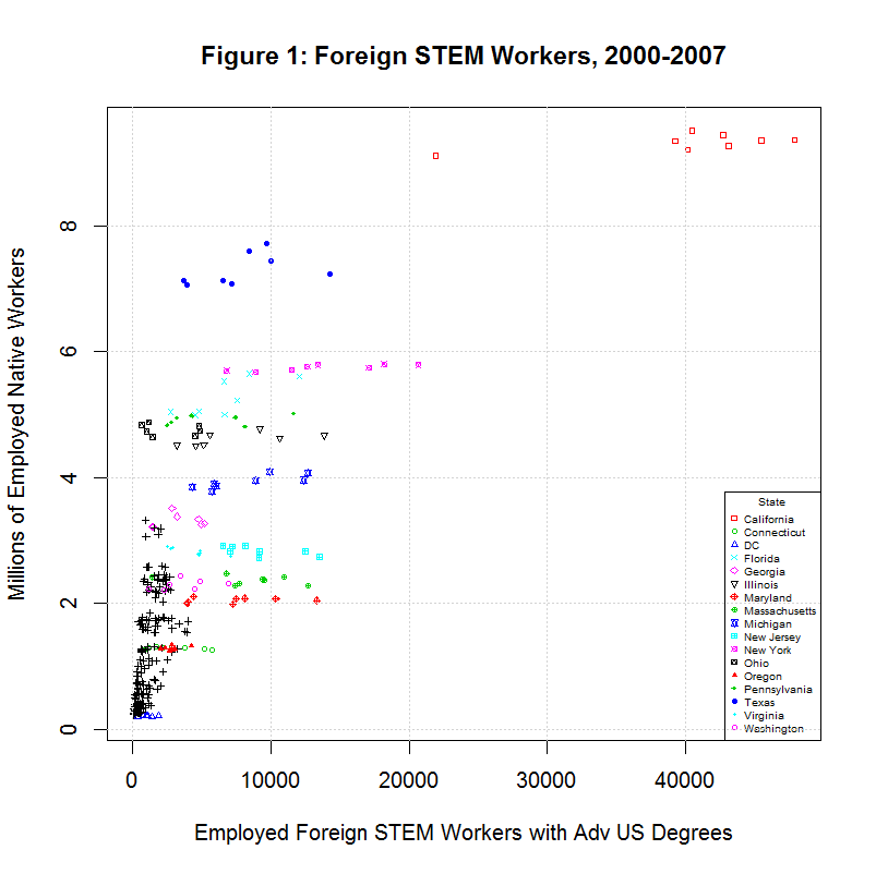
Before looking at the regression, it helps to look at the distribution of workers among the states in the following plot:
As can be seen, the largest number of foreign stem workers with advanced degrees from U.S. universities work in California. The following table shows the top ten states in the total of such workers from 2000 to 2007:
    TOTAL  STATE
---------  --------------
  320,974  California
  109,157  New York
   73,247  New Jersey
   65,901  Massachusetts
   65,797  Michigan
   63,745  Texas
   58,819  Maryland
   53,380  Florida
   52,153  Illinois
   44,441  Pennsylvania
---------  -------------
1,258,317  United States
As can be seen, California had nearly three times as many as the next highest state, New York, and over a quarter of the total in the United States. Also note that all of the labeled states varied much more in the percentage change of this group of foreign workers than in the percentage change of total employed native workers.
5. Initial Attempt at a Regression Fails Due to Zero Values
Now, we can create the variables for the regression by translating the indicated Stata statements to R as follows:
# Create emprate_native and immshare_emp_stem_e_grad plus their logs
dd$emprate_native             <- dd$emp_native / dd$pop_native * 100        # line 828
dd$immshare_emp_stem_e_grad   <- dd$emp_edus_stem_grad / dd$emp_total * 100 # line 858
dd$lnemprate_native           <- log(dd$emprate_native)                     # line 900
dd$lnimmshare_emp_stem_e_grad <- log(dd$immshare_emp_stem_e_grad)           # line 910
Now, we try an initial regression via the following R statement:
lm(lnemprate_native ~ lnimmshare_emp_stem_e_grad, data=dd)However, this results in the following error:
Error in lm.fit(x, y, offset = offset, singular.ok = singular.ok, ...) :
  NA/NaN/Inf in 'x'
Since 'x' in this regression is lnimmshare_emp_stem_e_grad, we can take a closer look at its value as follows:
> summary(dd$lnimmshare_emp_stem_e_grad)
   Min. 1st Qu.  Median    Mean 3rd Qu.    Max.
   -Inf    -Inf      -3    -Inf      -2       0
As can be seen, the problem appears to be that lnimmshare_emp_stem_e_grad contains values of minus infinity. This, is turn, can be traced back to the fact that immshare_emp_stem_e_grad contains values of zero since the natural log of zero is minus infinity. The zero values can be seen via the following R command:
> summary(dd$immshare_emp_stem_e_grad)
   Min. 1st Qu.  Median    Mean 3rd Qu.    Max.
0.00000 0.00000 0.07239 0.09963 0.14860 0.69780
The zero values can also be seen in the following plot of emprate_native versus immshare_emp_stem_e_grad:
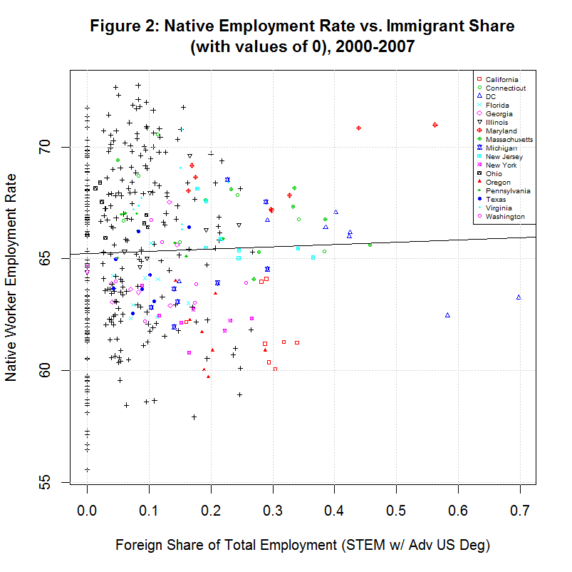
6. Problem with Study's Calculation of the Employment Rate
Note that the native worker employment rate plotted on the y-axis averages around 65 percent. This would imply an unemployment rate of 35 percent, much higher than the normally reported unemployment rate. According to Zavodny's execution file Tables1to3.do, the formula for this variable is as follows:
line 26: gen emp=(lfsr94<=2 & class94<=5)The following commands show the possible values of these variables from the original morg files at http://nber.org/morg/annual:
> mm <- read.dta("morg00.dta")
> levels(mm$lfsr94)
[1] "Employed-At Work"            "Employed-Absent"
[3] "Unemployed-On Layoff"        "Unemployed-Looking"
[5] "Retired-Not In Labor Force"  "Disabled-Not In Labor Force"
[7] "Other-Not In Labor Force"
> levels(mm$class94)
[1] "Government - Federal"          "Government - State"
[3] "Government - Local"            "Private, For Profit"
[5] "Private, Nonprofit"            "Self-Employed, Incorporated"
[7] "Self-Employed, Unincorporated" "Without Pay"
Hence, it appears that the native worker employment rate used by the study counts those not in the labor force, both retired and other, and the self-employed as unemployed in this number. This does not seem to be mentioned anywhere in the study as the term "native employment rate" appears 32 times but the terms "labor force" and "self-employed" do not appear once. This would seem to be a possible problem, especially the non-counting of the self-employed.
7. Removing Zero Values Changes Correlation in Regression from Positive to Negative
Getting back the zero values, the graph shows a large number of them. In fact, there are a total of 408 points (50 states plus D.C. times 8 years). About a quarter of those, 103 points, contain zero values for immshare_emp_stem_e_grad. In addition, the minimum non-zero value is 73.52493. This gap between the zero values and the next lowest value suggests that many, if not all, of the zero values are actually missing values. In fact, Zavodny's execution file Tables1to3.do contains the following lines, starting at line 807:
* replace missings with 0s
for var pop_edus_coll pop_nedus_coll pop_edus_grad pop_nedus_grad pop_edus_stem_coll pop_nedus_stem_coll pop_edus_stem_grad pop_nedus_stem_grad: replace X=0 if X==.
for var emp_edus_coll emp_nedus_coll emp_edus_grad emp_nedus_grad emp_edus_stem_coll emp_nedus_stem_coll emp_edus_stem_grad emp_nedus_stem_grad: replace X=0 if X==.
Hence, the code is explicitly setting missing values to zero. It's unclear why the program does this since missing values should be generally be treated as such and dropped from the analysis, not changed to some convenient value. Fortunately, Stata is able to handle these zero values. Page 264 of an article in the Stata Journal states:
The largest exponent (64 or 1024 for single and double precision, respectively) holds two different types of results, either what IEEE calls an infinity or what IEEE calls a “not-a-number” (NaN). Infinities have the largest exponent and zeros in the fraction. They can have a positive or a negative sign. Taking the logarithm of zero would result in a value of negative infinity. NaNs also have the highest exponent, but they have a nonzero fraction. A NaN is produced, for example, when one tries to take the logarithm of a negative number.
Stata does not report infinities or NaNs. Instead, Stata maps these values to missing. Stata takes up the largest positive power of two for its missing values. This means that all positive values that are stored in IEEE format with the exponent 1023 are recognized by Stata as missing.
Hence, it appears that Stata changes the zero values back to missing and removes them from the analysis. In any case, the following plot shows a plot of the natural logs of the values with the zero values removed:
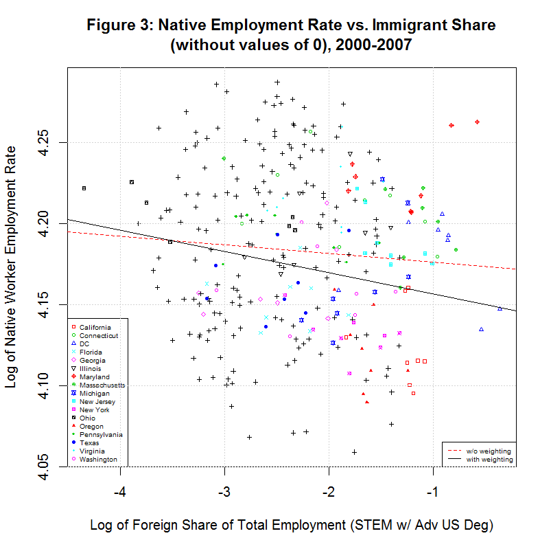
As can be seen, the values being correlated appear as a relatively random cloud of values. Still, a regression line can be fit to any set of data. The red line is a simple regression of the natural log of the native worker employment rate versus the natural log of the foreign STEM share (with advanced U.S. degrees) of total employment. The black line is a regression using a weighting used by Zavodny's in her study. Interestingly, both lines show a negative relation.
8. The Effect of Dummy or Indicator Variables on the Study
As mentioned above, following is the line in Zavodny's execution file that does the regression that we are trying to replicate:
xi: reg lnemprate_native lnimmshare_emp_stem_e_grad lnimmshare_emp_stem_n_grad i.statefip i.year [aw=weight_native] if year<2008, robust cluster(statefip)
As can be seen, the terms i.statefip and i.year appear among the arguments. These are dummy or indicator variables for the states and years, respectively. A short article titled "The Use of Dummy Variables in Regression Analysis" describes a dummy or indicator variable as "an artificial variable created to represent an attribute with two or more distinct categories/levels". Among things to keep in mind about dummy variables, it states that "the number of dummy variables necessary to represent a single attribute variable is equal to the number of levels (categories) in that variable minus one". For the eight years 2000 through 2007, seven dummy variables are required. Each of seven of the years will be indicated by having a unique one of the dummy variables set to one and the rest set to zero. The eighth year is the default and will be indicated if none of the seven indicators is set. Similarly, the 50 states plus D.C. will require 50 dummy variables.
The following plot shows the effect of using the state and/or year dummy variables in the weighted regression:
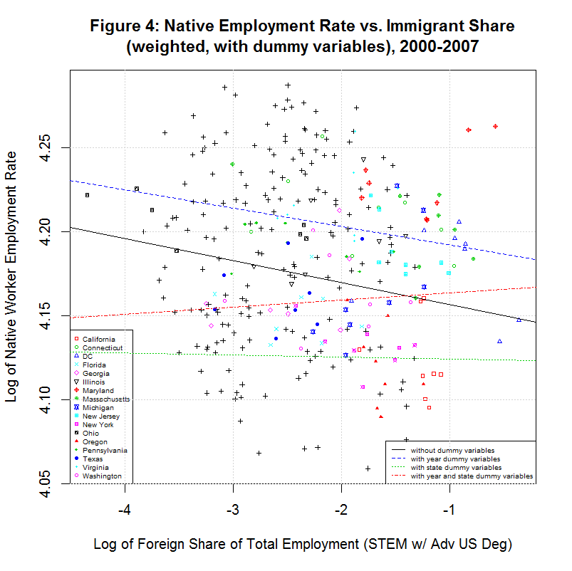
In addition, following table shows the properties of the four regression lines:
[1] "                          CORREL                                              "
[1] " N  INTERCEPT    SLOPE     COEF   P-VALUE  DESCRIPTION                        "
[1] "--  ---------  --------  -------  -------  -----------------------------------"
[1] "2000-2007, WEIGHTED WITH DUMMY VARIABLES"
[1] " 5)    4.1434   -0.0131  -0.0796   0.0002  without dummy variables"
[1] " 6)    4.1813   -0.0109  -0.0796   0.0012  with year dummy variables only"
[1] " 7)    4.1230   -0.0012  -0.0796   0.6701  with state dummy variables only"
[1] " 8)    4.1676    0.0042  -0.0796   0.0133  with year and state dummy variables"
As can be seen, all of the regression lines have negative slopes except for the last one which uses both the year and state dummy variables. This is the red line in the plot. In fact, the 0.0042 matches the 0.004 that in Table 2 of the study for "Advanced degree and in STEM occupation" in the column for US OLS. This is the number from which the claim that 2.62 native jobs are created as a result of each such foreign worker. Hence, this result absolutely depends upon the use of the dummy variables for both state and year. It is therefore critical to determine whether the use of these dummy variables is appropriate and is likely to give in a more accurate result than an alternate model that have fewer or more variables.
In fact, the addition of these dummy variables may be appropriate. As can be seen in the graph of the Native Employment Rate vs. Year in California below, the native employment rate went down sharply in 2002 and 2003, just after the tech crash and the 2001 recession. The model may therefore benefit from having a variable based on year to account for such nationwide economic events. Similarly, the model may benefit from a variable based on the state because some states may have a lower base employment rate than other states. This is especially due to the questionable definition of the employment rate defined in the study. It effectively counts retired people as unemployed so that states with large retired populations (like Florida) will likely have lower base employment rates.
However, just as the addition of dummy variables to account for the year and state may improve the model, so might the addition of others. The model for regression 8 above is essentially stating that all changes in the native employment rate that are not due to the year or state are due to the number of foreign-born students with an advanced degree from a U.S. university who stays to work in a STEM field. But how about other foreign-born workers? In fact, section 14 below suggests that the study is including at least some other groups of foreign workers. The effect of U.S. citizens with advanced degrees, however, appears not to be considered. After all, it would seem that if a foreign worker with an advanced degree would have a positive effect, so would an similarly skilled U.S. worker.
9. Use of Correlation Coefficients and P-Values
None of the data in the three plots above with regression lines appears to be very correlated to the naked eye. That shows one reason why it is useful to look at a plot of the data to see if there is some other visible relationship between the data. In addition, it's very important to look at the correlation coefficient and the p-value of any regression. The following table shows the y-intercept, slope, correlation coefficient, and p-value for each of the regressions discussed above, as calculated using the R language.
[1] "                          CORREL                                              "
[1] " N  INTERCEPT    SLOPE     COEF   P-VALUE  Y VARIABLE ~ X VARIABLE [, WEIGHTS]"
[1] "--  ---------  --------  -------  -------  -----------------------------------"
[1] "2000-2007, ALL DATA"
[1] " 1)   65.2318    1.0081   0.0310   0.5326  emprate_native ~ immshare_emp_stem_e_grad"
[1] "2000-2007, EXCLUDING POINTS WITH ZERO FOREIGN WORKERS IN STEM WITH ADVANCED US DEGREES"
[1] " 2)   65.9622   -2.4101  -0.0774   0.1777  emprate_native ~ immshare_emp_stem_e_grad"
[1] " 3)    4.1709   -0.0053  -0.0796   0.1654  lnemprate_native ~ lnimmshare_emp_stem_e_grad"
[1] " 4)    4.1434   -0.0131  -0.0796   0.0002  lnemprate_native ~ lnimmshare_emp_stem_e_grad, weights=weight_native"
[1] "                          CORREL                                              "
[1] " N  INTERCEPT    SLOPE     COEF   P-VALUE  DESCRIPTION                        "
[1] "--  ---------  --------  -------  -------  -----------------------------------"
[1] "2000-2007, WEIGHTED WITH DUMMY VARIABLES"
[1] " 5)    4.1434   -0.0131  -0.0796   0.0002  without dummy variables"
[1] " 6)    4.1813   -0.0109  -0.0796   0.0012  with year dummy variables only"
[1] " 7)    4.1230   -0.0012  -0.0796   0.6701  with state dummy variables only"
[1] " 8)    4.1676    0.0042  -0.0796   0.0133  with year and state dummy variables"
Correlation coefficients of -1 and 1 indicate the strongest possible negative and positive correlation and a correlation coefficient of 0 indicates the weakest possible correlation. The correlation coefficient obtained from the R cor function gives the unweighted correlation between just two variables. That is why regressions 3 through 8 above all have the same correlation coefficient. They are all measuring the correlation between the log of the native employment rate (lnemprate_native) and the immigrant share (immshare_emp_stem_e_grad) which is not affected by weighting or additional variables. In any event, the coefficient shows that these two variables have little correlation.
The p-value is the standard method that statisticians use to measure the "significance" of their analyses. Wikipedia defines it as follows:
In statistics, the p-value is a function of the observed sample results (a statistic) that is used for testing a statistical hypothesis. Before performing the test a threshold value is chosen, called the significance level of the test, traditionally 5% or 1% [1] and denoted as alpha. If the p-value is equal or smaller than the significance level (alpha), it suggests that the observed data are inconsistent with the assumption that the null hypothesis is true, and thus that hypothesis must be rejected and the alternative hypothesis is accepted as true. When the p-value is calculated correctly, such a test is guaranteed to control the Type I error rate to be no greater than alpha.
Table 2 of the study showed that the regression on which the 2.6 job claim is made had a p-value such that 0.05 < p-value < 0.1. Following is one rough description of how to interpret a p-value:
0.10  < P          No evidence against the null hypothesis. The data appear to be consistent with the null hypothesis.
0.05  < P < 0.10   Weak evidence against the null hypothesis in favor of the alternative.
0.01  < P < 0.05   Moderate evidence against the null hypothesis in favor of the alternative.
0.001 < P < 0.01   Strong evidence against the null hypothesis in favor of the alternative.
        P < 0.001  Very strong evidence against the null hypothesis in favor of the alternative.
The author gives qualifiers to these definitions. Still, the claim's regression provided "weak evidence" according to this definition. In any case, the only regressions in the table above that are deemed to be significant are those numbered 4 through 8. All of these use the weighting used by Zavodny's in the study and the last three use dummy variables, making them "multivariable regressions". One problem with weighting and multivariable regressions is that the quality of the model is no longer clearly visible in the scatter plots and the correlation coefficient.
10. Removing the Effects of Year and State from the Scatter Plot
The slope in regression 8 above closely matches the 0.004 figure on which the study bases its 2.6 job claim. However, this is based on a weighted regression with three independent variables (immigrant share, year, and state). It is theoretically possible that the apparent lack of correlation in the scatter plot in Figure 4 is due to the year and/or state and not immigrant share (of STEM workers with advanced US degrees). In fact, it is possible to remove the predicted effects of the year and state from the scatter plot by doing an unweighted regression with the three variables. That regression is shown as regression 9 in the following table:
[1] "                          CORREL                                              "
[1] " N  INTERCEPT    SLOPE     COEF   P-VALUE  DESCRIPTION                        "
[1] "--  ---------  --------  -------  -------  -----------------------------------"
[1] "2000-2007, NATIVE WORKER EMPLOYMENT RATE ADJUSTED TO REMOVE EFFECTS OF YEAR AND STATE"
[1] " 9)    4.1550   0.00176  -0.0796   0.3028  with year and state dummy variables, unweighted"
[1] "10)    4.1550   0.00176   0.1017   0.0761  native employment rate adjusted to remove effects of year and state"
[1] "11)    4.1565   0.00242   0.1017   0.0081  native employment rate adjusted to remove effects of
Passing the result of this regression to the summary function gives coefficients for the following formula:
y = c1*im + c2*y1 + c3*y2 + ... + c8*y8 + c9*s2 + c10*s3 + ... + c58*s51

where y  = predicted log of native employment rate
      cN = coefficients
      im = log of immigrant share (of STEM workers with advanced US degrees)
      yN = 1 if data point is for year N, otherwise set to 0
      sN = 1 if data point is for state N, otherwise set to 0
The predicted effect of the year and state can then be removed by subtracting all but the first term (c1*im) in the above equation from the y-values in the scatter plot. That results in the following plot:
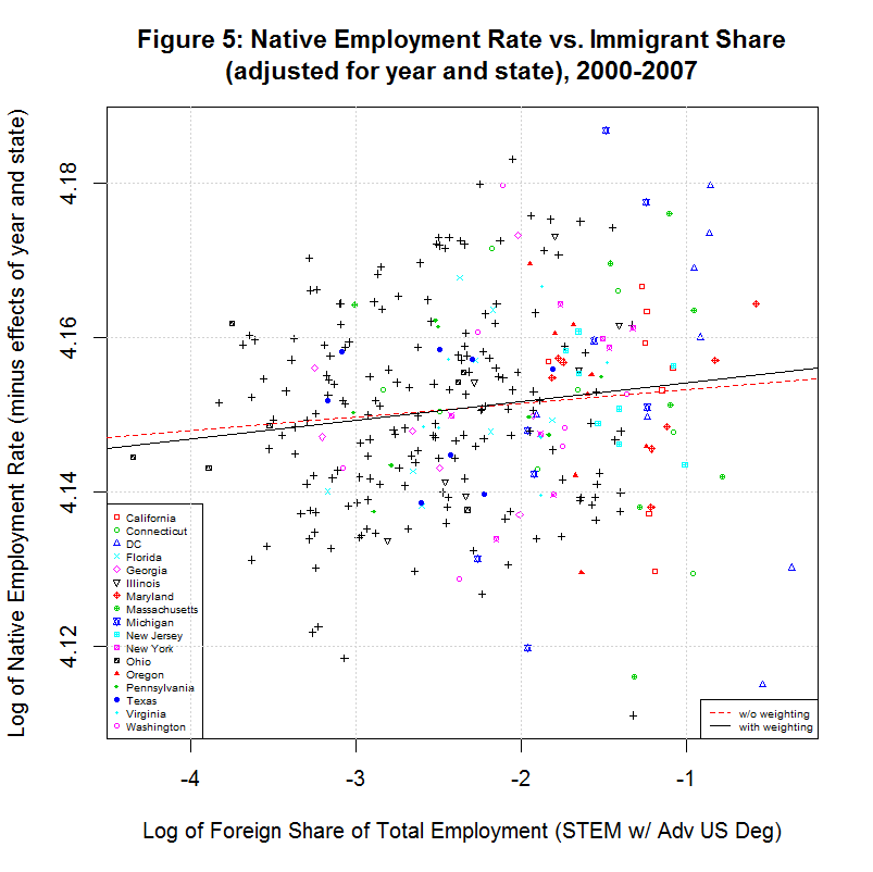
The red and black lines are the unweighted and weighted regression lines based on the adjusted data. Their coefficients are shown in regressions 10 and 11 in the table above. Note that the unweighted regression (10) has the exact same intercept and slope as the multivariable regression (9). This indicates that the adjustment was done correctly. The correlation coefficient is different because the data has been adjusted, backing out the predicted effect of the year and state. Both the low value of the correlation coefficient and the visible appearance of the adjusted data show that there is little correlation between the native employment rate and the immigrant share, even after accounting for the year and state.
11. Removing the Effects of Year from the Scatter Plot
Because of the lack of correlation, it would be instructive to look at some of the key states individually. It would still seem advisable to remove the apparent effect of the year. We can repeat the process of the prior section but apply it to just the year, not the year and state, by doing an unweighted regression with the immigrant share and the year. That regression is shown as regression 12 in the following table:
[1] "                          CORREL                                              "
[1] " N  INTERCEPT    SLOPE     COEF   P-VALUE  DESCRIPTION                        "
[1] "--  ---------  --------  -------  -------  -----------------------------------"
[1] "2000-2007, NATIVE WORKER EMPLOYMENT RATE ADJUSTED TO REMOVE EFFECTS OF YEAR ONLY"
[1] "12)    4.2015  -0.00315  -0.0796   0.3961  with year dummy variable, unweighted"
[1] "13)    4.2015  -0.00315  -0.0499   0.3855  native employment rate adjusted to remove effects of year"
[1] "14)    4.1737  -0.01079  -0.0499   0.0010  native employment rate adjusted to remove effects of
Passing the result of this regression to the summary function gives coefficients for the following formula:
y = c1*im + c2*y1 + c3*y2 + ... + c8*y8

where y  = predicted log of native employment rate
      cN = coefficients
      im = log of immigrant share (of STEM workers with advanced US degrees)
      yN = 1 if data point is for year N, otherwise set to 0
The predicted effect of the year can then be removed by subtracting all but the first term (c1*im) in the above equation from the y-values in the scatter plot. That results in the following plot:
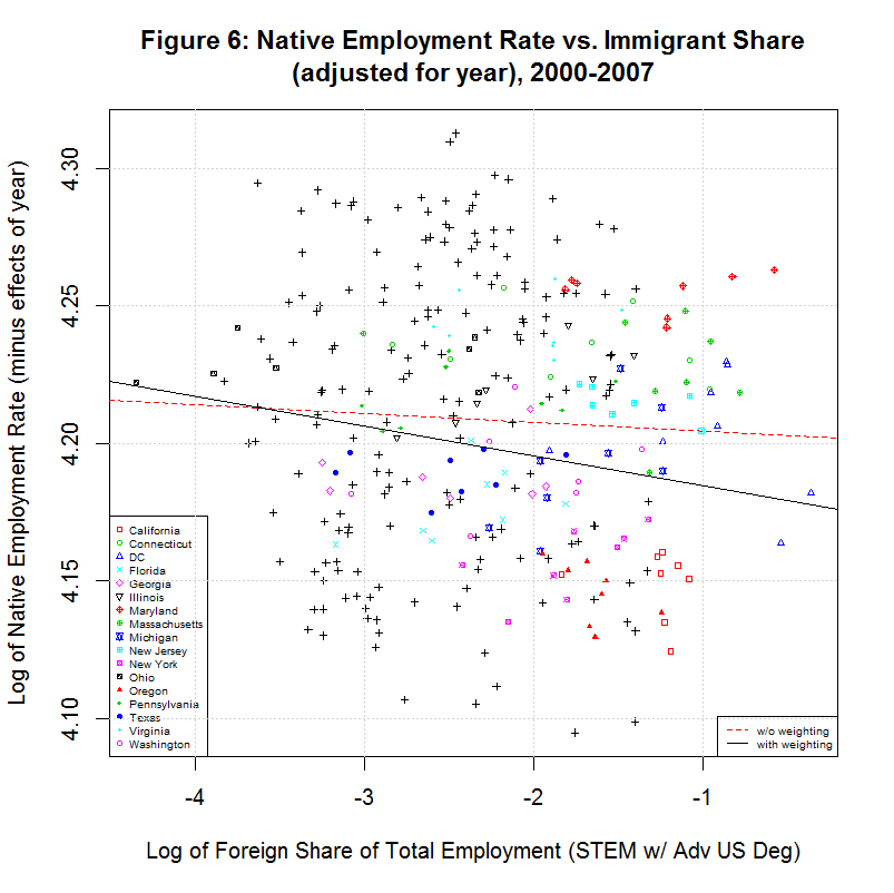
The red and black lines are the unweighted and weighted regression lines based on the adjusted data. Their coefficients are shown in regressions 13 and 14 in the table above. As before, note that the unweighted regression (13) has the exact same intercept and slope as the multivariable regression (12). This indicates that the adjustment was done correctly.
Because the data is no longer adjusted for state, it's now possible to see the difference between the base native employment rate of some of the key states. As can be seen, California and Oregon have among the lowest and Maryland is among the highest. Also of note is that the slope of both the weighted and unweighted regression lines are now negative, countering the key finding of the study. To get a better idea of what is going on, however, it's useful to look at the individual states.
12. Looking at the States Individually
The following table shows the results of regressions for each of the 17 states listed in the legends of the previous plots. It uses the year-adjusted data obtained in the previous section. These 17 states include the 16 states that had the largest number of foreign-born STEM workers with advanced US degrees from 2000 to 2007. They also include the District of Columbia since it had the largest share of such workers as a percentage of total employment.
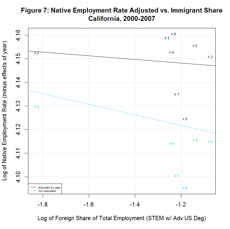
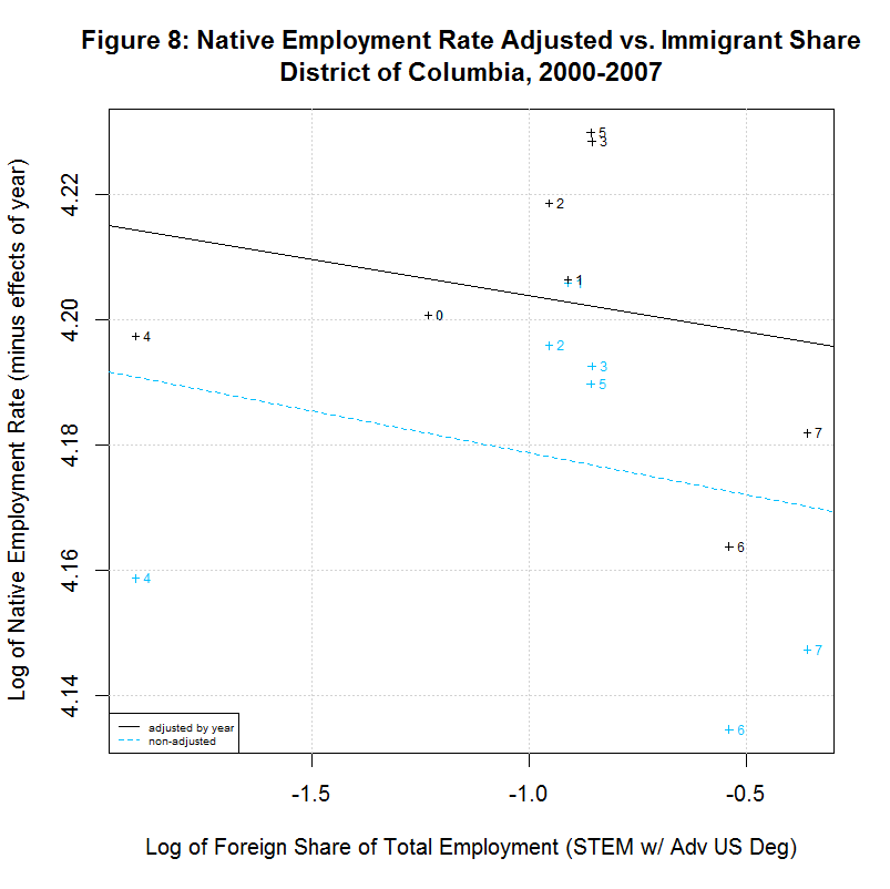
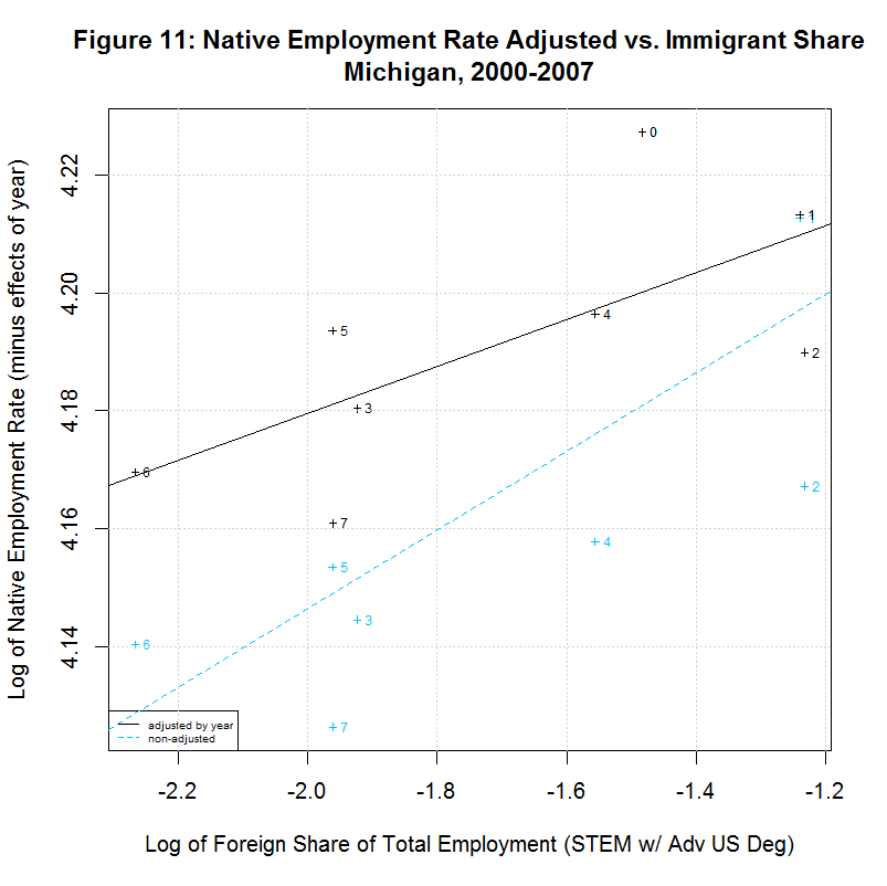
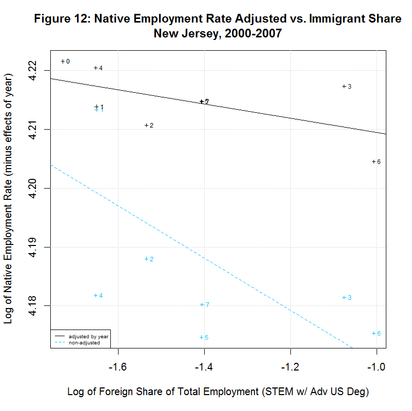
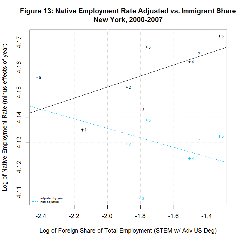
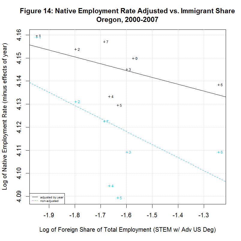
[1] "                          CORREL                                              "
[1] " N  INTERCEPT    SLOPE     COEF   P-VALUE  DESCRIPTION                        "
[1] "--  ---------  --------  -------  -------  -----------------------------------"
[1] "2000-2007, NATIVE WORKER EMPLOYMENT RATE (YEAR-ADJUSTED) VS IMMIGRANT SHARE, BY STATE"
[1] "15)    4.1388   -0.0078  -0.1446   0.7326  California"
[1] "16)    4.2274   -0.0046  -0.2416   0.5643  Connecticut"
[1] "17)    4.1924   -0.0115  -0.2359   0.5738  District of Columbia"
[1] "18)    4.2179    0.0167   0.5133   0.1933  Florida"
[1] "19)    4.1975    0.0034   0.1708   0.7142  Georgia"
[1] "20)    4.2704    0.0238   0.8411   0.0177  Illinois"
[1] "21)    4.2578    0.0020   0.1246   0.7688  Maryland"
[1] "22)    4.2183   -0.0066  -0.2383   0.5699  Massachusetts"
[1] "23)    4.2593    0.0399   0.6928   0.0568  Michigan"
[1] "24)    4.1974   -0.0121  -0.5969   0.1182  New Jersey"
[1] "25)    4.1964    0.0222   0.6356   0.0903  New York"
[1] "26)    4.2350    0.0016   0.1583   0.7346  Ohio"
[1] "27)    4.0970   -0.0297  -0.5362   0.1707  Oregon"
[1] "28)    4.2289    0.0051   0.2701   0.5177  Pennsylvania"
[1] "29)    4.1927    0.0013   0.0703   0.8687  Texas"
[1] "30)    4.2413   -0.0011  -0.0405   0.9242  Virginia"
[1] "31)    4.2068    0.0077   0.2468   0.5936  Washington"
As can be seen, 7 of the states had negative slopes (and correlation coefficients) and 10 had positive slopes. Six had correlation cofficients above 0.5 and the plots of these six are shown in Figures 9 to 14 at the bottom of this page. Also included is the District of Columbia which had the largest share and California which had the largest number of such workers. California seems especially important to look at since it had nearly three times the number of such workers as the next highest state, New York, and over a quarter of the total in the United States.
All of the plots contain the data and regression line for the year-adjusted data in black and the non-adjusted data in blue. The numbers next to the data indicate the year with 0 to 7 indicating 2000 to 2007. The data point for 2000 is identical for both sets of data and the data point for 2001 is nearly identical. This is because 2000 is the base year and 2001 had a very small coefficient in regression 12. The other years have adjusted numbers that are noticably higher than the unadjusted numbers. This is likely adjusting for the large drop in the native employment rate after 2001 due to the recession.
As can be seen in the plot for California, there is a negative slope to the regression line, countering the key finding of the study. Also, the labels show that the native employment rate was generally dropping in California from 2000 to 2007. The same negative slope can be seen in the District of Columbia though the steady drop in the native employment rate seen in California is not seen there.
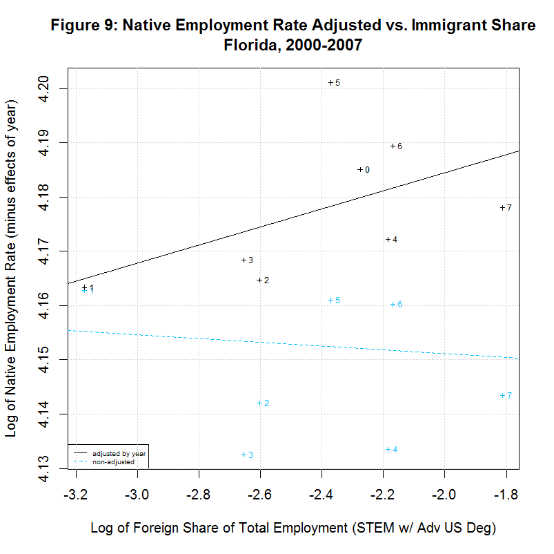
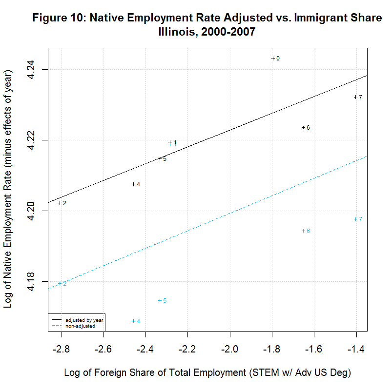
The plots for Florida, Illinois, and Michigan show regression lines with positive slopes. However, the labels of the points show a key difference between those states. In Florida, the native employment rate and immigrant share dropped sharply from 2000 to 2001 but climbed back steadily through 2007, surpassing its 2000 levels. The same was true in Illinois except that the drop covered two years, from 2000 to 2002. In Michigan, however, the trend has been generally downward since 2001, hitting a low in 2006 with only a small recovery in 2007. This brings up a key point. The study purports to find a positive correlation between the native employment rate and the immigrant share and imply that this indicates that an increase in the immigrant share has a positive effect on the native employment rate. Even when there is a positive correlation, however, these plots show that the movement is often in reverse, with both variables shrinking. It is doubtful that this study would hold the decrease in Michigan gives evidence that such foreign workers create native jobs. It much more likely indicates that an economic slowdown in the state is causing a drop in both variables.
In any event, Florida shows a situation similar to New York in that the regression line is positive for the adjusted data but is negative for the unadjusted data. This is likely due to the fact that both states show the immigrant share generally increasing over time with 2000 and/or 2001 at the left side of the plot. Adjusting the employment rate up for years 2002 to 2007 (which are toward the right side of the plot) tends to move the regression line up. The final two states, New Jersey and Oregon, both show a negative correlation. Both show a general increase in the immigrant share since 2000 or 2001 but both show a reversal in 2007.
Looking at the individual states shows that, whatever correlation there may or may not be on the national level, there is often a very different situation in key states. Any such correlation is of little help to workers in California where over a quarter of such workers are located. In addition, when both variables are shrinking, it seems very unlikely that a positive correlation reveals anything about how the growth of one variable will affect the other.
The R summary function provides a number of statistics for any regression. Among those included are the Multiple R-Squared, Adjusted R-Squared, F-Statistic, and p-value. Following are those statistics for the regressions in this analysis:
[1] "     MULTIPLE   ADJUSTED      F-                                    "
[1] " N  R-SQUARED  R-SQUARED  STATISTIC  DF1/DF2   P-VALUE   DESCRIPTION"
[1] "--  ---------  ---------  ---------  -------  ---------  -----------"
[1] "2000-2007, ALL DATA"
[1] " 1)    0.0010    -0.0015     0.3902    1/406  5.326e-01  emprate_native ~ immshare_emp_stem_e_grad"
[1] "2000-2007, EXCLUDING POINTS WITH ZERO FOREIGN WORKERS IN STEM WITH ADVANCED US DEGREES"
[1] " 2)    0.0060     0.0027     1.8254    1/303  1.777e-01  emprate_native ~ immshare_emp_stem_e_grad"
[2] " 3)    0.0063     0.0031     1.9337    1/303  1.654e-01  lnemprate_native ~ lnimmshare_emp_stem_e_grad"
[3] " 4)    0.0443     0.0411    14.0325    1/303  2.151e-04  lnemprate_native ~ lnimmshare_emp_stem_e_grad, weights=weight_native"
[1] "2000-2007, WEIGHTED WITH DUMMY VARIABLES"
[1] " 5)    0.0443     0.0411    14.0325    1/303  2.151e-04  without dummy variables"
[2] " 6)    0.1884     0.1664     8.5870    8/296  1.152e-03  with year dummy variables only"
[3] " 7)    0.8113     0.7750    22.3727   49/255  6.701e-01  with state dummy variables only"
[4] " 8)    0.9386     0.9247    67.6517   56/248  1.326e-02  with year and state dummy variables"
[1] "2000-2007, NATIVE WORKER EMPLOYMENT RATE ADJUSTED TO REMOVE EFFECTS OF YEAR AND STATE"
[1] " 9)    0.9329     0.9177    61.5384   56/248  3.028e-01  with year and state dummy variables, unweighted"
[2] "10)    0.0103     0.0071     3.1674    1/303  7.612e-02  native employment rate adjusted to remove effects of year and state"
[3] "11)    0.0229     0.0197     7.1045    1/303  8.101e-03  native employment rate adjusted to remove effects of year and state, weighted"
[1] "2000-2007, NATIVE WORKER EMPLOYMENT RATE ADJUSTED TO REMOVE EFFECTS OF YEAR ONLY"
[1] "12)    0.0992     0.0749     4.0748    8/296  3.961e-01  with year dummy variable, unweighted"
[2] "13)    0.0025    -0.0008     0.7551    1/303  3.855e-01  native employment rate adjusted to remove effects of year"
[3] "14)    0.0353     0.0321    11.0963    1/303  9.721e-04  native employment rate adjusted to remove effects of year, weighted"
[1] ""
[1] "      MULTIPLE   ADJUSTED      F-                                    "
[1] "  N  R-SQUARED  R-SQUARED  STATISTIC  DF1/DF2   P-VALUE   DESCRIPTION"
[1] "---  ---------  ---------  ---------  -------  ---------  -----------"
[1] "2000-2007, NATIVE WORKER EMPLOYMENT RATE (YEAR-ADJUSTED) VS IMMIGRANT SHARE, BY STATE"
 [1] "15)    0.0209    -0.1423     0.1281    1/  6  7.326e-01  California"
 [2] "16)    0.0584    -0.0986     0.3720    1/  6  5.643e-01  Connecticut"
 [3] "17)    0.0556    -0.1017     0.3535    1/  6  5.738e-01  District of Columbia"
 [4] "18)    0.2634     0.1407     2.1460    1/  6  1.933e-01  Florida"
 [5] "19)    0.0292    -0.1650     0.1503    1/  5  7.142e-01  Georgia"
 [6] "20)    0.7075     0.6490    12.0949    1/  5  1.770e-02  Illinois"
 [7] "21)    0.0155    -0.1486     0.0946    1/  6  7.688e-01  Maryland"
 [8] "22)    0.0568    -0.1004     0.3611    1/  6  5.699e-01  Massachusetts"
 [9] "23)    0.4800     0.3934     5.5392    1/  6  5.678e-02  Michigan"
[10] "24)    0.3563     0.2491     3.3217    1/  6  1.182e-01  New Jersey"
[11] "25)    0.4039     0.3046     4.0661    1/  6  9.034e-02  New York"
[12] "26)    0.0251    -0.1699     0.1285    1/  5  7.346e-01  Ohio"
[13] "27)    0.2875     0.1688     2.4215    1/  6  1.707e-01  Oregon"
[14] "28)    0.0729    -0.0816     0.4720    1/  6  5.177e-01  Pennsylvania"
[15] "29)    0.0049    -0.1609     0.0298    1/  6  8.687e-01  Texas"
[16] "30)    0.0016    -0.1648     0.0098    1/  6  9.242e-01  Virginia"
[17] "31)    0.0609    -0.1269     0.3243    1/  5  5.936e-01  Washington"
[1] ""
[1] "     MULTIPLE   ADJUSTED      F-                                    "
[1] " N  R-SQUARED  R-SQUARED  STATISTIC  DF1/DF2   P-VALUE   DESCRIPTION"
[1] "--  ---------  ---------  ---------  -------  ---------  -----------"
[1] "2000-2007, OLS WITH YEAR, STATE, AND SPECIFIED GROUP OF FOREIGN WORKERS"
[1] "32)    0.9386     0.9247    67.6517   56/248  1.326e-02  Advanced US degree and in STEM occupation"
[2] "33)    0.9347     0.9210    68.2801   57/272  3.623e-01  Advanced foreign degree and in STEM occupation"
[3] "34)    0.9369     0.9211    59.1447   54/215  1.409e-02  Advanced US|foreign degree and in STEM occupation"
[4] "35)    0.9374     0.9258    80.7031   57/307  1.476e-02  Advanced degree and in STEM occupation"
[5] "36)    0.9383     0.9279    90.4313   58/345  7.973e-05  Advanced degree"
[6] "20)    0.9354     0.9247    87.1543   58/349  4.442e-02  Bachelor's degree or higher"
[7] "38)    0.9376     0.9272    89.4368   58/345  5.346e-04  Advanced degree and NOT in STEM occupation"
[8] "39)    0.9350     0.9241    86.2585   58/348  2.255e-01  Bachelor's degree only"
[1] "2000-2007, OLS WITH YEAR, STATE, AND 4 SUBSETS OF FOREIGN WORKERS WITH BACHELOR'S DEGREE OR HIGHER"
[1] "40)    0.9385     0.9223    58.0543   56/213  2.260e-02  OLS with Year, State, and 4 Subsets"
[2] "41)    0.9347     0.9240    87.8415   57/350  3.907e-05  OLS with Year and State only"
To this point, this analysis has dealt only with the study's finding regarding foreign-born workers who earned an advanced degree in the U.S. and then worked in STEM fields. Doing the same OLS regressions on other groups of foreign workers gave the following results:
[1] "                          CORREL                                                             "
[1] " N  INTERCEPT    SLOPE     COEF   P-VALUE  T.R.C    OLS   Y VARIABLE ~ X VARIABLE [, WEIGHTS]"
[1] "--  ---------  --------  -------  -------  -----  ------  -----------------------------------"
[1] "2000-2007, OLS WITH YEAR, STATE, AND SPECIFIED GROUP OF FOREIGN WORKERS"
[1] "32)    4.1676    0.0042  -0.0796   0.0133  3.3.1   0.004  Advanced US degree and in STEM occupation"
[1] "33)    4.1601    0.0016   0.0783   0.3623  3.3.3 -0.0002  Advanced foreign degree and in STEM occupation"
[1] "34a)   4.1690    0.0045  -0.0640   0.0141  3.3.1   0.004  Advanced US degree and in STEM occupation"
[1] "34b)   4.1690   -0.0002  -0.0640   0.9118  3.3.3 -0.0002  Advanced foreign degree and in STEM occupation"
[1] "35)    4.1640    0.0041   0.0680   0.0148  1.4.1   0.004  Advanced degree and in STEM occupation"
[1] "36)    4.1682    0.0111   0.2092   0.0001  1.3.1   0.011  Advanced degree"
[1] "37)    4.1596    0.0079   0.1841   0.0444  1.2.1   0.008  Bachelor's degree or higher"
[1] "38)    4.1678    0.0086   0.2242   0.0005  .....  ......  Advanced degree and NOT in STEM occupation"
[1] "39)    4.1551   -0.0039   0.1926   0.2255  .....  ......  Bachelor's degree only"

* T.R.C = Table.Row.Column
Regression 32 is repeat of regression 8 above and the slope of 0.0042 matches the 0.004 in column 1, row 3 (counting only the blue rows) in Table 2 in the study. However, the slope of 0.0016 for regression 33 does not match the -0.0002 in column 3, row 3 in Table 2. Looking again at the code for the regression from line 998 of the study's execution file shows that both of these variables were members of the same regression. Regression 34 includes both of these variables and the slopes for both variables do match the values from the study. Regressions 35, 36, and 37 can likewise be seen to match the values from the study. The last two regressions were not done in the study except in combination with other groups.
In the last section, all of the OLS regressions assumed a model with variables for year, state, and a selected group of foreign workers. It would seem reasonable to put these groups into a single multi-variable regression, providing the groups are independent and do not overlap. Following is the results of such a regression:
[1] "                          CORREL                                              "
[1] " N  INTERCEPT    SLOPE     COEF   P-VALUE  DESCRIPTION                        "
[1] "--  ---------  --------  -------  -------  -----------------------------------"
[1] "2000-2007, OLS WITH YEAR, STATE, AND 4 SUBSETS OF FOREIGN WORKERS WITH BACHELOR'S DEGREE OR HIGHER"
[1] "40a)   4.1703    0.0041  -0.0640   0.0226  Advanced US degree and in STEM occupation"
[1] "40b)   4.1703   -0.0002  -0.0640   0.9340  Advanced foreign degree and in STEM occupation"
[1] "40c)   4.1703    0.0079  -0.0640   0.0606  Advanced degree and NOT in STEM occupation"
[1] "40d)   4.1703   -0.0091  -0.0640   0.0838  Bachelor's degree only"
Line 40d shows what might be called a "fallacy of composition" that is implied by the study. Table 1 shows a positive slope of 0.008 for foreign workers with a bachelor's degree or higher. This might mislead someone to think that a positive correlation exists for ALL foreign workers with such degrees. In fact, item 40d shows a strong negative slope for foreign workers who have only a bachelor's degree. That is, by the study's reasoning, such workers are associated with a decrease in native jobs.
It is also worth noting that the slope of a variable can vary depending on what other variables are included in the regression. In regression 32, foreign workers with advanced US degree and working in a STEM occupation have a slope of 0.0042. That jumped to nearly 0.0045 when one other group of foreign workers were included but dropped to 0.0041 when three other groups were included.
16. First and Last Year are Critical to Results
On page 8, the study states the following:
This paper uses data from the US Census Bureau’s Current Population Survey (CPS) covering all fifty states and the District of Columbia, focusing on the periods 2000–2007 and 2000–2010. The former represents a period of economic recovery and growth while the latter period includes the recent recession, during which the US-born employment rate fell by more than two percentage points. The analysis begins in 2000 to avoid including the hightech bubble of the late 1990s.
This seems to be the study's rationale for looking at 2000 to 2007. Regarding periods of "economic recovery and growth", the following table shows the growth in the study's key data from 2000 to 2013:
year   emp_imm   emp_native    emp_total   pop_native  imm_level  nat_level  ln_imm_level  ln_nat_level
----  --------  -----------  -----------  -----------  ---------  ---------  ------------  ------------
2000   148,984  103,082,363  119,167,108  154,182,309  0.1250216   66.85745     -2.079268      4.202563
2001   141,657  102,771,951  119,489,933  155,359,951  0.1185521   66.15086     -2.132403      4.191938
2002   121,521  101,993,592  118,798,501  157,039,250  0.1022919   64.94783     -2.279925      4.173584
2003   151,761  101,737,445  119,047,895  159,092,173  0.1274797   63.94874     -2.059798      4.158082
2004   156,425  102,441,401  120,166,278  160,589,716  0.1301738   63.79076     -2.038885      4.155608
2005   176,080  104,113,290  122,534,825  162,270,376  0.1436980   64.16038     -1.940042      4.161386
2006   175,012  105,253,440  124,517,864  163,469,261  0.1405517   64.38730     -1.962180      4.164916
2007   186,874  105,904,192  125,808,429  164,786,302  0.1485389   64.26759     -1.906909      4.163056
2008   185,667  105,480,298  124,964,666  165,699,739  0.1485759   63.65749     -1.906659      4.153517
2009   203,877  101,483,644  120,106,722  167,119,661  0.1697470   60.72514     -1.773446      4.106358
2010   177,485  100,668,333  119,534,797  167,863,135  0.1484805   59.97048     -1.907302      4.093852
2011   160,208  101,328,629  120,445,461  168,384,994  0.1330134   60.17676     -2.017305      4.097286
2012   199,521  102,432,985  122,263,732  168,723,889  0.1631893   60.71042     -1.812844      4.106115
2013   207,956  103,388,318  123,574,162  169,356,101  0.1682847   61.04788     -1.782098      4.111659
The following table shows the results of regressions on the study's data:
[1] "                           JOBS    CORREL                                     "
[1] " N  INTERCEPT    SLOPE   CREATED    COEF   DESCRIPTION                        "
[1] "--  ---------  --------  -------  -------  -----------------------------------"
[1] "2000-2007, ALL DATA"
[1] " 1)   -0.4284   -0.0073   -481.1  -0.0640  ln_nat_level ~ ln_imm_level + ln_imm_level2"
[1] " 2)   -0.3998   -0.0054   -356.0  -0.0640  ln_nat_level ~ ln_imm_level + ln_imm_level2 + fyear"
[1] " 3)   -0.4316    0.0021    137.3  -0.0640  ln_nat_level ~ ln_imm_level + ln_imm_level2 + fyear + floc"
[1] " 4)   -0.4167    0.0040    263.0  -0.0640  ln_nat_level ~ ln_imm_level + ln_imm_level2 + fyear + floc, weights=weight"
[1] "USING STUDY'S FORMULA"
[1] " 5)   -0.4167    0.0045    293.4  -0.0640  2000-2007, study's data with corrected job count"
[1] " 6)   -0.5193   -0.0005    -32.2  -0.0299  2002-2005, during first span of increasing immigrant level"
[1] " 7)   -0.4772   -0.0036   -198.2  -0.1662  2006-2009, during second  span of increasing immigrant level"
[1] " 8)   -0.4862   -0.0020   -121.1  -0.1111  2002-2009, during increasing immigrant level (except 2005-06)"
Regressions 1 to 4 show the results of the regression after adding each additional variable. The variable fyear is a dummy variable for year, floc is a dummy variable for the state, and weight is a weight used by the study. The weight is based on the native population of each state in each year. Regression 4 is the one on which the study's 262 number is based. The calculation value was actually just under 263 and the study appears to truncate it to 262. This value, in turn, appears to be based on a truncated value for the slope of 0.004. When using the exact slope, shown to be about 0.0045 above, I came up with a calculated job gain of 293. However, regressions 6 through 8 show that when looking at periods of growth in the level of the foreign stem worker being studied, the level of native workers dropped according to the study's formula.
The following tables show the slopes obtained for all time spans containing 4 or more years between 2000 and 2013 and the corresponding native jobs gained or lost:
SLOPE BETWEEN GIVEN YEARS (using same regression as was used to obtain 262 job finding)
---- ------- ------- ------- ------- ------- ------- ------- ------- ------- ------- -------  ----
Year    2003    2004    2005    2006    2007    2008    2009    2010    2011    2012    2013  Year
---- ------- ------- ------- ------- ------- ------- ------- ------- ------- ------- -------  ----
2000  0.0034  0.0043  0.0040  0.0038  0.0045  0.0025  0.0015  0.0018  0.0025  0.0036  0.0038  2000
2001 .......  0.0044  0.0038  0.0036  0.0043  0.0018  0.0008  0.0012  0.0019  0.0031  0.0033  2001
2002 ....... ....... -0.0005 -0.0009  0.0005 -0.0018 -0.0020 -0.0011 -0.0002  0.0012  0.0017  2002
2003 ....... ....... ....... -0.0006  0.0001 -0.0027 -0.0027 -0.0019 -0.0008  0.0009  0.0014  2003
2004 ....... ....... ....... ....... -0.0012 -0.0035 -0.0030 -0.0022 -0.0010  0.0009  0.0013  2004
2005 ....... ....... ....... ....... ....... -0.0058 -0.0044 -0.0034 -0.0020  0.0001  0.0007  2005
2006 ....... ....... ....... ....... ....... ....... -0.0036 -0.0030 -0.0020  0.0002  0.0009  2006
2007 ....... ....... ....... ....... ....... ....... .......  0.0002  0.0006  0.0025  0.0024  2007
2008 ....... ....... ....... ....... ....... ....... ....... ....... -0.0005  0.0015  0.0013  2008
2009 ....... ....... ....... ....... ....... ....... ....... ....... .......  0.0019  0.0016  2009
2010 ....... ....... ....... ....... ....... ....... ....... ....... ....... .......  0.0026  2010

JOBS GAINED/LOST BETWEEN GIVEN YEARS (using same regression as was used to obtain 262 job finding but with truncation errors)
---- ------- ------- ------- ------- ------- ------- ------- ------- ------- ------- -------  ----
Year    2003    2004    2005    2006    2007    2008    2009    2010    2011    2012    2013  Year
---- ------- ------- ------- ------- ------- ------- ------- ------- ------- ------- -------  ----
2000  217.89  284.32  274.93  269.32  262.99# 129.20  125.53  124.35  124.53  245.06  241.05  2000
2001 .......  286.29  274.57  268.11  261.14  128.14   62.13   61.55  123.40  182.06  179.01  2001
2002 ....... .......    0.00  -66.03    0.00 -126.06 -122.07  -60.54    0.00   59.80  117.60  2002
2003 ....... ....... .......  -62.73    0.00 -181.70 -176.36 -117.05  -59.01   58.14   57.26  2003
2004 ....... ....... ....... .......  -60.16 -178.35 -172.89 -115.00  -58.15   57.31   56.45  2004
2005 ....... ....... ....... ....... ....... -348.87 -225.22 -169.11 -114.48    0.00   55.60  2005
2006 ....... ....... ....... ....... ....... ....... -222.57 -167.55 -113.87    0.00   55.19  2006
2007 ....... ....... ....... ....... ....... ....... .......    0.00   56.32  110.86  109.06  2007
2008 ....... ....... ....... ....... ....... ....... ....... .......    0.00   55.18   54.18  2008
2009 ....... ....... ....... ....... ....... ....... ....... ....... .......  109.54  107.33  2009
2010 ....... ....... ....... ....... ....... ....... ....... ....... ....... .......  164.18  2010

NATIVE JOBS GAINED/LOST PER EACH 100 STEM WORKERS WITH ADVANCED US DEGREES BETWEEN GIVEN YEARS (using study's methodology with no errors)
---- ------- ------- ------- ------- ------- ------- ------- ------- ------- ------- -------  ----
Year    2003    2004    2005    2006    2007    2008    2009    2010    2011    2012    2013  Year
---- ------- ------- ------- ------- ------- ------- ------- ------- ------- ------- -------  ----
2000  245.51  306.94  274.79  257.13  293.44* 158.33   96.35  112.38  154.98  221.82  225.99  2000
2001 .......  317.81  262.67  242.41  280.19  114.42   46.88   73.19  117.79  188.00  194.49  2001
2002 ....... .......  -32.21  -59.12   30.37 -110.55 -121.07  -65.43  -12.20   74.36   98.75  2002
2003 ....... ....... .......  -39.24    3.18 -162.83 -161.62 -108.66  -47.03   50.47   78.46  2003
2004 ....... ....... ....... .......  -70.56 -206.88 -175.46 -125.54  -57.93   52.45   72.69  2004
2005 ....... ....... ....... ....... ....... -338.56 -249.66 -189.44 -114.91    4.97   41.33  2005
2006 ....... ....... ....... ....... ....... ....... -198.23 -168.66 -115.45    8.89   50.58  2006
2007 ....... ....... ....... ....... ....... ....... .......   13.27   33.91  136.92  132.92  2007
2008 ....... ....... ....... ....... ....... ....... ....... .......  -27.36   82.76   73.07  2008
2009 ....... ....... ....... ....... ....... ....... ....... ....... .......  101.55   83.93  2009
2010 ....... ....... ....... ....... ....... ....... ....... ....... ....... .......  142.78  2010

# value is 262.99 if the slope is truncated.
* value is 293.44 if the slope is not truncated.
The table above shows that when one looks at a time span for which the foreign worker being studied is increasing, a loss of native jobs is indicated. For example, 2002 to 2009 shows an steady increase in such workers and their share of the employment pool was generally increasing. The table, however, shows a negative slope of -0.0020 during this period, indicating a loss of native jobs.
The following table shows the p-values that correspond to the slopes in the prior tables:
P-VALUE OF REGRESSION SLOPE BETWEEN GIVEN YEARS (using study's methodology)
---- ------- ------- ------- ------- ------- ------- ------- ------- ------- ------- -------  ----
Year    2003    2004    2005    2006    2007    2008    2009    2010    2011    2012    2013  Year
---- ------- ------- ------- ------- ------- ------- ------- ------- ------- ------- -------  ----
2000  0.1144  0.0206  0.0307  0.0492  0.0141  0.1631  0.3987  0.3366  0.1956  0.0487  0.0313  2000
2001 .......  0.0425  0.0685  0.0993  0.0330  0.3439  0.6955  0.5476  0.3426  0.1038  0.0688  2001
2002 ....... .......  0.8532  0.7291  0.8360  0.3923  0.3364  0.6081  0.9247  0.5321  0.3633  2002
2003 ....... ....... .......  0.8374  0.9840  0.2334  0.2242  0.4175  0.7269  0.6815  0.4818  2003
2004 ....... ....... ....... .......  0.7145  0.1782  0.2313  0.3912  0.6894  0.6844  0.5275  2004
2005 ....... ....... ....... ....... .......  0.0544  0.1336  0.2368  0.4618  0.9707  0.7241  2005
2006 ....... ....... ....... ....... ....... .......  0.2731  0.3076  0.4641  0.9470  0.6584  2006
2007 ....... ....... ....... ....... ....... ....... .......  0.9417  0.8395  0.3188  0.2376  2007
2008 ....... ....... ....... ....... ....... ....... ....... .......  0.8900  0.5667  0.5138  2008
2009 ....... ....... ....... ....... ....... ....... ....... ....... .......  0.4249  0.4028  2009
2010 ....... ....... ....... ....... ....... ....... ....... ....... ....... .......  0.2039  2010
In the above table, the p-values are colored red if they are less than 0.01 (p < 0.01), orange if they are less than 0.05 (0.01 <= p < 0.05), and green if they are less than 0.1 (0.05 <= p < 0.1). As can be seen, there are no red values of the highest significance but there 8 and 4 of the other two levels, respectively. There is at least one span, 2005 to 2008, that has a p-value less than 0.1 but corresponds to native jobs losses of 348.87 and 338.56 in the prior two tables.
In any event, these numbers show how critical the first and last year of the chosen time span are to the results. This seems to be especially true for certain years such as the tech crash that occurred in 2000-2002. As can be seen in the first table in this section, there was a steep job loss for both foreign and native workers during this period. This underlines an interesting fact. A job increase for both foreign and native workers will result in a regression finding a positive association between the two. However, a steep job loss will result in a regression finding a similar positive association. Since time is not included in the plot, both cases are essentially identical from a mathematical point of view. Of course, the study is not claiming that foreign job LOSSES lead to native job LOSSES. Hence, it makes sense to focus on periods of gains in the jobs of foreign workers. As mentioned above, when looking at periods of growth in the level of the foreign stem worker being studied, the level of native workers generally dropped according to the study's formula.
The following table shows the standard errors that correspond to the slopes in the prior tables:
STANDARD ERROR OF REGRESSION SLOPE BETWEEN GIVEN YEARS (using study's methodology)
---- ------- ------- ------- ------- ------- ------- ------- ------- ------- ------- -------  ----
Year    2003    2004    2005    2006    2007    2008    2009    2010    2011    2012    2013  Year
---- ------- ------- ------- ------- ------- ------- ------- ------- ------- ------- -------  ----
2000  0.0021  0.0018  0.0018  0.0019  0.0018  0.0018  0.0018  0.0019  0.0019  0.0018  0.0017  2000
2001 .......  0.0022  0.0021  0.0022  0.0020  0.0019  0.0019  0.0020  0.0020  0.0019  0.0018  2001
2002 ....... .......  0.0026  0.0026  0.0023  0.0020  0.0021  0.0021  0.0021  0.0020  0.0018  2002
2003 ....... ....... .......  0.0030  0.0026  0.0022  0.0023  0.0023  0.0023  0.0021  0.0019  2003
2004 ....... ....... ....... .......  0.0032  0.0026  0.0025  0.0025  0.0025  0.0022  0.0020  2004
2005 ....... ....... ....... ....... .......  0.0030  0.0029  0.0028  0.0027  0.0024  0.0021  2005
2006 ....... ....... ....... ....... ....... .......  0.0032  0.0029  0.0028  0.0024  0.0021  2006
2007 ....... ....... ....... ....... ....... ....... .......  0.0033  0.0030  0.0025  0.0021  2007
2008 ....... ....... ....... ....... ....... ....... ....... .......  0.0035  0.0026  0.0021  2008
2009 ....... ....... ....... ....... ....... ....... ....... ....... .......  0.0023  0.0019  2009
2010 ....... ....... ....... ....... ....... ....... ....... ....... ....... .......  0.0020  2010
As can be seen, the standard error is between 0.0017 and 0.0022 in the first two rows that correspond to job gains and between 0.0017 and 0.0033 when including all of the spans that correspond to job gains. This compares to 0.0020 and 0.0035 for those spans that correspond to job losses, a relatively small difference.
17. Correlation Does Not Imply Causation
It is worth repeating the oft-repeated phrase that "correlation does not imply causation". As stated at this link, there are at least five possibilities when events A and B are correlated:
But one of the fundamental challenges when using cross-state comparisons to show a relationship between immigrants and jobs is that immigrants tend to be more mobile and go where the jobs are. As a result, evidence of high immigrant shares in states with strong economic growth and high employment could be the result of greater job opportunities (as immigrants move to jobs), rather than the cause.
The author is stating that "B may be the cause of A" as stated in possibility 2 above. She then continues:
Cross-state comparisons would then show an artificially high impact of immigrants on the native employment rate. The study avoids “overcounting” the effects of immigrant workers drawn by a recent economic boom by using an estimation technique (known as “two-stage least squares (2SLS) regression estimation” and discussed in the appendix) that is designed to yield the effect of immigration independent of recent growth and employment opportunities.
The problem is, the study does not use a 2SLS regression to obtain the 262 number. As shown in the first table on this page, the 0.004 slope that was used came from an OLS regression because the 0.0004 slope obtained by the 2SLS regression was not significant. Hence, by the author's own standards, this study has not taken steps to avoid "overcounting" in this case. The study does avoid causal language in the following case (bold added):
However, it then gets bolder with the following statements (bold added):
However, it then just states outright causation in the following statements (bold added):
These last three statement of causation are in the largest typeface. In any case, the media, at least those who support increasing the supply of such workers, usually use outright causal language. As stated above, the following statements are from a FWD.us video and the Facebook home page of Compete America (bold added):
It might be useful to conclude this discussion with the following statement from the aforementioned link:
Correlation is a valuable type of scientific evidence in fields such as medicine, psychology, and sociology. But first correlations must be confirmed as real, and then every possible causative relationship must be systematically explored. In the end correlation can be used as powerful evidence for a cause-and-effect relationship between a treatment and benefit, a risk factor and a disease, or a social or economic factor and various outcomes. But it is also one of the most abused types of evidence, because it is easy and even tempting to come to premature conclusions based upon the preliminary appearance of a correlation.
The general conclusion of this analysis is that Zavodny's own numbers do not support the claim that "every additional 100 foreign- born workers who earned an advanced degree in the United States and then worked in STEM fields led to an additional 262 jobs for US natives" for the following reasons:
The study relies on the fact that the percentage of the workforce that is foreign born—the immigrant share—varies from state to state. This difference across states allows for comparisons that yield the relationship between immigration and American jobs. But one of the fundamental challenges when using cross-state comparisons to show a relationship between immigrants and jobs is that immigrants tend to be more mobile and go where the jobs are. As a result, evidence of high immigrant shares in states with strong economic growth and high employment could be the result of greater job opportunities (as immigrants move to jobs), rather than the cause. Cross-state comparisons would then show an artificially high impact of immigrants on the native employment rate. The study avoids “overcounting” the effects of immigrant workers drawn by a recent economic boom by using an estimation technique (known as “two-stage least squares (2SLS) regression estimation” and discussed in the appendix) that is designed to yield the effect of immigration independent of recent growth and employment opportunities.
Hence by its own definition, the study is not attempting to avoid "overcounting the effects of immigrant workers drawn by a recent economic boom" in the calculation of the 262 number since it is not using 2SLS regression in this case.
In addition, following are some broader pointers that can be taken from this analysis regarding other studies:
Increase opportunities for immigrants to enter the United States workforce — and for foreign students to stay in the United States to work — so that we can attract and keep the best, the brightest and the hardest-working, who will strengthen our economy;
This would suggest that this group only searches out and/or funds research that supports this principle. In fact, their online Research & Reports page list a number of reports, all seemingly favorable toward increased immigration.