Once again, the analysis here looked at a specific claim made in a study titled "Immigration and American Jobs", written by economist Madeline Zavodny and published by the American Enterprise Institute and the Partnership For A New American Economy. The claim is made on page 10 of the study as follows:
During 2000– 2007, a 10 percent increase in the share of such workers boosted the US-born employment rate by 0.04 percent. Evaluating this at the average numbers of foreign- and US-born workers during that period, this implies that every additional 100 foreign- born workers who earned an advanced degree in the United States and then worked in STEM fields led to an additional 262 jobs for US natives. (See Table 2)
The analysis here then showed how the author's data could be reproduced almost precisely from the original US Census Bureau’s Current Population Survey (CPS) data at http://nber.org/morg/annual. As stated, the advantage of this is that it verifies the author's data and allows the data to be updated and for additional variables to be derived. This analysis does this last item, updating the data through 2013 and deriving a new, arguably more meaningful, measure of the native worker employment rate.
25. Updating the Study Through 2013
The data is extracted from the CPS data files via the R program morg13lf.R. The lf in the filename indicates that the program is now extracting a variable that indicates if the person is in the labor force. This value is derived from the CPS variable lfsr94 which can have the following values:
Following are all of the key differences between morg07.R and morg13lf.R:
26. Slope of Key Regression Cut in Half and Significance of First 3 Regressions Increased
Following is a table showing the same regressions that were run on the 2000-2007 data:
[1] "                          CORREL                                              "
[1] " N  INTERCEPT    SLOPE     COEF   P-VALUE  Y VARIABLE ~ X VARIABLE [, WEIGHTS]"
[1] "--  ---------  --------  -------  -------  -----------------------------------"
[1] "2000-2013, ALL DATA"
[1] " 1)   94.3599   -3.0597  -0.1526   0.0000  emprate_native ~ immshare_emp_stem_e_grad"
[1] "2000-2013, EXCLUDING POINTS WITH ZERO FOREIGN WORKERS IN STEM WITH ADVANCED US DEGREES"
[1] " 2)   94.3670   -3.0926  -0.1501   0.0004  emprate_native ~ immshare_emp_stem_e_grad"
[1] " 3)    4.5332   -0.0040  -0.1308   0.0020  lnemprate_native ~ lnimmshare_emp_stem_e_grad"
[1] " 4)    4.5281   -0.0051  -0.1308   0.0002  lnemprate_native ~ lnimmshare_emp_stem_e_grad, weights=weight_native"
[1] "--  ---------  --------  -------  -------  -----------------------------------"
[1] "                          CORREL                                              "
[1] " N  INTERCEPT    SLOPE     COEF   P-VALUE  DESCRIPTION                        "
[1] "--  ---------  --------  -------  -------  -----------------------------------"
[1] "2000-2013, WEIGHTED WITH DUMMY VARIABLES"
[1] " 5)    4.5281   -0.0051  -0.1308   0.0002  without dummy variables"
[1] " 6)    4.5598   -0.0026  -0.1308   0.0000  with year dummy variables only"
[1] " 7)    4.5336   -0.0046  -0.1308   0.0001  with state dummy variables only"
[1] " 8)    4.5734    0.0020  -0.1308   0.0000  with year and state dummy variables"
[1] "2000-2013, NATIVE WORKER EMPLOYMENT RATE ADJUSTED TO REMOVE EFFECTS OF YEAR AND STATE"
[1] " 9)    4.5681   0.00155  -0.1308   0.0000  with year and state dummy variables, unweighted"
[1] "10)    4.5681   0.00155   0.1307   0.0020  native employment rate adjusted to remove effects of year and state"
[1] "11)    4.5679   0.00145   0.1307   0.0038  native employment rate adjusted to remove effects of year and state, weighted"
[1] "2000-2013, NATIVE WORKER EMPLOYMENT RATE ADJUSTED TO REMOVE EFFECTS OF YEAR ONLY"
[1] "12)    4.5583  -0.00300  -0.1308   0.0000  with year dummy variable, unweighted"
[1] "13)    4.5583  -0.00300  -0.1544   0.0003  native employment rate adjusted to remove effects of year"
[1] "14)    4.5555  -0.00288  -0.1544   0.0001  native employment rate adjusted to remove effects of year, weighted"
[1] "2000-2013, NATIVE WORKER EMPLOYMENT RATE (YEAR-ADJUSTED) VS IMMIGRANT SHARE, BY STATE"
[1] "15)    4.5387   -0.0069  -0.1021   0.7285  California"
[1] "16)    4.5641   -0.0017  -0.0729   0.8044  Connecticut"
[1] "17)    4.5541    0.0090   0.5385   0.0469  District of Columbia"
[1] "18)    4.5447   -0.0094  -0.3175   0.2687  Florida"
[1] "19)    4.5653    0.0017   0.0992   0.7471  Georgia"
[1] "20)    4.5468   -0.0031  -0.2121   0.4867  Illinois"
[1] "21)    4.5725   -0.0011  -0.0752   0.7983  Maryland"
[1] "22)    4.5635   -0.0048  -0.4285   0.1264  Massachusetts"
[1] "23)    4.6022    0.0336   0.6688   0.0089  Michigan"
[1] "24)    4.5536   -0.0051  -0.2032   0.4859  New Jersey"
[1] "25)    4.5643    0.0013   0.0648   0.8258  New York"
[1] "26)    4.5466   -0.0035  -0.5361   0.0724  Ohio"
[1] "27)    4.5414   -0.0049  -0.1633   0.5769  Oregon"
[1] "28)    4.5588   -0.0027  -0.3750   0.1864  Pennsylvania"
[1] "29)    4.5921    0.0122   0.8692   0.0001  Texas"
[1] "30)    4.5862    0.0025   0.2292   0.4307  Virginia"
[1] "31)    4.5610    0.0023   0.2442   0.4213  Washington"
[1] "--  ---------  --------  -------  -------  -----  ------  -----------------------------------"
[1] "                          CORREL                                                             "
[1] " N  INTERCEPT    SLOPE     COEF   P-VALUE  T.R.C    OLS   DESCRIPTION                        "
[1] "--  ---------  --------  -------  -------  -----  ------  -----------------------------------"
[1] "2000-2013, OLS WITH YEAR, STATE, AND SPECIFIED GROUP OF FOREIGN WORKERS"
[1] "32)    4.5719    0.0020  -0.1308   0.0000  3.3.1   0.004  Advanced US degree and in STEM occupation"
[1] "33)    4.5613    0.0005  -0.1089   0.0000  3.3.3 -0.0002  Advanced foreign degree and in STEM occupation"
[1] "34a)   4.5717    0.0021  -0.1301   0.0000  3.3.1   0.004  Advanced US degree and in STEM occupation"
[1] "34b)   4.5717    0.0005  -0.1301   0.0814  3.3.3 -0.0002  Advanced foreign degree and in STEM occupation"
[1] "35)    4.5658    0.0015  -0.1091   0.0000  1.4.1   0.004  Advanced degree and in STEM occupation"
[1] "36)    4.5632    0.0005  -0.2262   0.0000  1.3.1   0.011  Advanced degree"
[1] "37)    4.5630    0.0017  -0.2341   0.0000  1.2.1   0.008  Bachelor's degree or higher"
[1] "38)    4.5635    0.0007  -0.2303   0.0000  .....  ......  Advanced degree and NOT in STEM occupation"
[1] "39)    4.5637    0.0010  -0.2168   0.0000  .....  ......  Bachelor's degree only"
[1] "--  ---------  --------  -------  -------  -----------------------------------"
[1] "                          CORREL                                              "
[1] " N  INTERCEPT    SLOPE     COEF   P-VALUE  DESCRIPTION                        "
[1] "--  ---------  --------  -------  -------  -----------------------------------"
[1] "2000-2013, OLS WITH YEAR, STATE, AND 4 SUBSETS OF FOREIGN WORKERS WITH BACHELOR'S DEGREE OR HIGHER"
[1] "40a)   4.5733    0.0021  -0.1310   0.0000  Advanced US degree and in STEM occupation"
[1] "40b)   4.5733    0.0005  -0.1310   0.0795  Advanced foreign degree and in STEM occupation"
[1] "40c)   4.5733   -0.0000  -0.1310   0.0000  Advanced degree and NOT in STEM occupation"
[1] "40d)   4.5733    0.0017  -0.1310   0.0057  Bachelor's degree only"
As can be seen, the slope of the key regression (8) has decreased from 0.0042 to 0.0020. Less noticable is the fact that the p-values for the first three regressions is far lower than before, indicating higher significance. As previously mentioned, the main differences between this and the study's variables is that this run extended the span of the study from 2000-2007 to 2000-2013 and the employment rate has been fixed (or, at least, arguably improved). To judge the contribution of both changes, following is a run over the same period but using the study's original definition of the native employment rate:
[1] "                          CORREL                                              "
[1] " N  INTERCEPT    SLOPE     COEF   P-VALUE  Y VARIABLE ~ X VARIABLE [, WEIGHTS]"
[1] "--  ---------  --------  -------  -------  -----------------------------------"
[1] "2000-2013, ALL DATA"
[1] " 1)   63.8884    0.3060   0.0086   0.8191  emprate_native ~ immshare_emp_stem_e_grad"
[1] "2000-2013, EXCLUDING POINTS WITH ZERO FOREIGN WORKERS IN STEM WITH ADVANCED US DEGREES"
[1] " 2)   64.5348   -2.5183  -0.0724   0.0912  emprate_native ~ immshare_emp_stem_e_grad"
[1] " 3)    4.1454   -0.0064  -0.0801   0.0618  lnemprate_native ~ lnimmshare_emp_stem_e_grad"
[1] " 4)    4.1095   -0.0172  -0.0801   0.0000  lnemprate_native ~ lnimmshare_emp_stem_e_grad, weights=weight_native"
[1] "--  ---------  --------  -------  -------  -----------------------------------"
[1] "                          CORREL                                              "
[1] " N  INTERCEPT    SLOPE     COEF   P-VALUE  DESCRIPTION                        "
[1] "--  ---------  --------  -------  -------  -----------------------------------"
[1] "2000-2013, WEIGHTED WITH DUMMY VARIABLES"
[1] " 5)    4.1095   -0.0172  -0.0801   0.0000  without dummy variables"
[1] " 6)    4.1780   -0.0123  -0.0801   0.0000  with year dummy variables only"
[1] " 7)    4.0791   -0.0095  -0.0801   0.0000  with state dummy variables only"
[1] " 8)    4.1600    0.0034  -0.0801   0.0000  with year and state dummy variables"
[1] "2000-2013, NATIVE WORKER EMPLOYMENT RATE ADJUSTED TO REMOVE EFFECTS OF YEAR AND STATE"
[1] " 9)    4.1488   0.00092  -0.0801   0.0000  with year and state dummy variables, unweighted"
[1] "10)    4.1488   0.00092   0.0389   0.3644  native employment rate adjusted to remove effects of year and state"
[1] "11)    4.1502   0.00157   0.0389   0.1117  native employment rate adjusted to remove effects of year and state, weighted"
[1] "2000-2013, NATIVE WORKER EMPLOYMENT RATE ADJUSTED TO REMOVE EFFECTS OF YEAR ONLY"
[1] "12)    4.1983  -0.00450  -0.0801   0.0313  with year dummy variable, unweighted"
[1] "13)    4.1983  -0.00450  -0.0654   0.1272  native employment rate adjusted to remove effects of year"
[1] "14)    4.1672  -0.01269  -0.0654   0.0000  native employment rate adjusted to remove effects of year, weighted"
[1] "2000-2013, NATIVE WORKER EMPLOYMENT RATE (YEAR-ADJUSTED) VS IMMIGRANT SHARE, BY STATE"
[1] "15)    4.0863   -0.0356  -0.2849   0.3236  California"
[1] "16)    4.2400    0.0025   0.0978   0.7393  Connecticut"
[1] "17)    4.2242    0.0093   0.1438   0.6239  District of Columbia"
[1] "18)    4.1489   -0.0086  -0.2183   0.4533  Florida"
[1] "19)    4.1886    0.0063   0.1930   0.5275  Georgia"
[1] "20)    4.2503    0.0163   0.5614   0.0459  Illinois"
[1] "21)    4.2644    0.0063   0.2682   0.3540  Maryland"
[1] "22)    4.2213   -0.0075  -0.2515   0.3858  Massachusetts"
[1] "23)    4.2454    0.0440   0.4330   0.1220  Michigan"
[1] "24)    4.1822   -0.0196  -0.6495   0.0119  New Jersey"
[1] "25)    4.1884    0.0149   0.3904   0.1676  New York"
[1] "26)    4.2163   -0.0020  -0.1358   0.6740  Ohio"
[1] "27)    4.1199   -0.0166  -0.3182   0.2675  Oregon"
[1] "28)    4.2261    0.0011   0.0664   0.8216  Pennsylvania"
[1] "29)    4.2182    0.0100   0.4586   0.0991  Texas"
[1] "30)    4.2536    0.0011   0.0331   0.9107  Virginia"
[1] "31)    4.1974   -0.0000  -0.0002   0.9996  Washington"
[1] "--  ---------  --------  -------  -------  -----  ------  -----------------------------------"
[1] "                          CORREL                                                             "
[1] " N  INTERCEPT    SLOPE     COEF   P-VALUE  T.R.C    OLS   Y VARIABLE ~ X VARIABLE [, WEIGHTS]"
[1] "--  ---------  --------  -------  -------  -----  ------  -----------------------------------"
[1] "2000-2013, OLS WITH YEAR, STATE, AND SPECIFIED GROUP OF FOREIGN WORKERS"
[1] "32)    4.1629    0.0035  -0.0801   0.0000  3.3.1   0.004  Advanced US degree and in STEM occupation"
[1] "33)    4.1507    0.0002  -0.0017   0.0000  3.3.3 -0.0002  Advanced foreign degree and in STEM occupation"
[1] "34a)   4.1643    0.0038  -0.0791   0.0000  3.3.1   0.004  Advanced US degree and in STEM occupation"
[1] "34b)   4.1643   -0.0002  -0.0791   0.6080  3.3.3 -0.0002  Advanced foreign degree and in STEM occupation"
[1] "35)    4.1559    0.0026   0.0053   0.0000  1.4.1   0.004  Advanced degree and in STEM occupation"
[1] "36)    4.1539    0.0039   0.0518   0.0000  1.3.1   0.011  Advanced degree"
[1] "37)    4.1511    0.0034   0.0311   0.0000  1.2.1   0.008  Bachelor's degree or higher"
[1] "38)    4.1534    0.0027   0.0422   0.0000  .....  ......  Advanced degree and NOT in STEM occupation"
[1] "39)    4.1493   -0.0013   0.0369   0.0000  .....  ......  Bachelor's degree only"
[1] "--  ---------  --------  -------  -------  -----------------------------------"
[1] "                          CORREL                                              "
[1] " N  INTERCEPT    SLOPE     COEF   P-VALUE  DESCRIPTION                        "
[1] "--  ---------  --------  -------  -------  -----------------------------------"
[1] "2000-2013, OLS WITH YEAR, STATE, AND 4 SUBSETS OF FOREIGN WORKERS WITH BACHELOR'S DEGREE OR HIGHER"
[1] "40a)   4.1572    0.0038  -0.0809   0.0000  Advanced US degree and in STEM occupation"
[1] "40b)   4.1572   -0.0002  -0.0809   0.5771  Advanced foreign degree and in STEM occupation"
[1] "40c)   4.1572   -0.0023  -0.0809   0.0000  Advanced degree and NOT in STEM occupation"
[1] "40d)   4.1572   -0.0052  -0.0809   0.0000  Bachelor's degree only"
As can be seen, extending the study alone decreased the regression 8 from 0.0042 to 0.0034. However, the fixing of the native employment rate lowered it by a greater amount, to 0.0020 and greatly lowered the p-values of the first three regressions. Hence, it had the larger effect.
27. An Initial Look at the Data
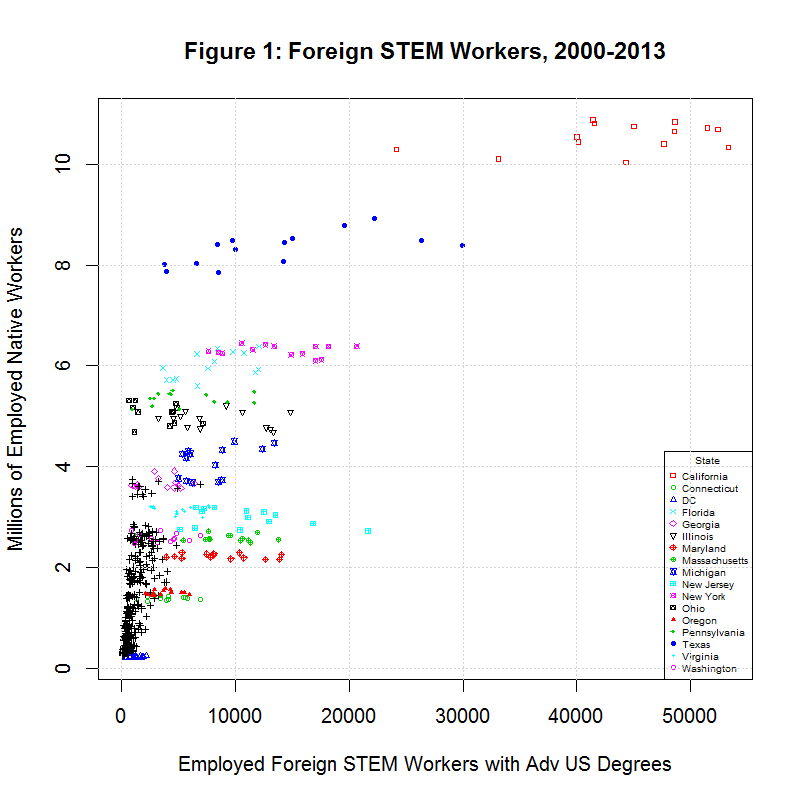
Before looking at the regression lines, it helps to look at the distribution of workers among the states in the following plot:
As can be seen, the largest number of foreign stem workers with advanced degrees from U.S. universities worked in California in 2000 to 2013. In fact, the total number of such workers who worked in each state during that period can be found by running the following R statement after running amjobs13lf.R:
aggregate(dd$emp_edus_stem_grad, by=list(dd$st), FUN=sum, na.rm=FALSE)The following table shows the top ten states in the total of such workers from 2000 to 2007 and from 2000 to 2013:
2000-2007  STATE           2000-2013  STATE
---------  --------------  ---------  --------------
  320,974  California        611,900  California
  109,157  New York          194,356  New York
   73,247  New Jersey        192,497  Texas
   65,901  Massachusetts     150,325  New Jersey
   65,797  Michigan          125,395  Massachusetts
   63,745  Texas             121,739  Maryland
   58,819  Maryland          111,728  Illinois
   53,380  Florida           110,608  Florida
   52,153  Illinois          109,980  Michigan
   44,441  Pennsylvania       78,661  Pennsylvania
---------  -------------   ---------  -------------
1,258,317  United States   2,487,977  United States
As can be seen, California now has over three times as many as the next highest state, New York, and just under a quarter of the total in the United States, similar to before. One noticable change is that Texas has risen from 6th to 3rd, just behind New York. As before, note that all of the labeled states varied much more in the percentage change of this group of foreign workers than in the percentage change of total employed native workers.
28. Regression with Corrected Employment Rate Shows Negative Correlation
As before, the following plots look at the values and the logs of the native worker employment rate and the share of total employment held by the foreign stem workers in question. Following are the R statements which calculate these variables:
# Create emprate_native and immshare_emp_stem_e_grad plus their logs
dd$emprate_native             <- dd$emp_native / dd$lf_native * 100
dd$immshare_emp_stem_e_grad   <- dd$emp_edus_stem_grad / dd$emp_total * 100
dd$lnemprate_native           <- log(dd$emprate_native)
dd$lnimmshare_emp_stem_e_grad <- log(dd$immshare_emp_stem_e_grad)
These formulas are the same as they were for the 2000 to 2007 period with one exception. The native worker employment rate is now calculated by dividing the number of employed natives by the number of natives in the labor force rather than by the total native population as was done previously. However, the immigrant share has also changed somewhat due to the fact that the definition of employment has change and now includes those who are self-employed. In any event, the next plot looks at the first two of these variables:
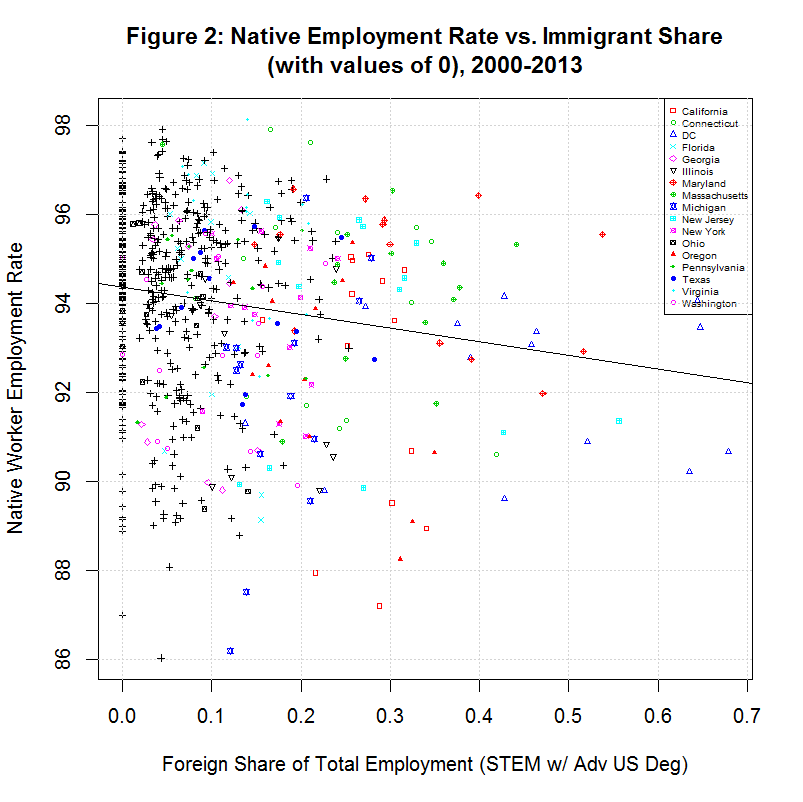
One noticable difference between this plot and the corresponding one for 2000-2007 is that the native worker employment rate in this one is between 92 and 95 percent, corresponding to an unemployment rate between 5 and 8 percent. For 2000 to 2007, however, the employment rate was between 65 and 66 percent, corresponding to an unemployment rate between 34 and 35 percent. Hence, this measure of the employment rate is much closer to what most people would expect. More importantly, it is not affected by changes in the labor force such as the effect of the Baby Boomer retirement.
As before, a vertical column of zeroes can be seen on the left side of the plot. These represent data points for which there were no samples that could be classified as a foreign stem worker with an advanced degree from a U.S. university. The R program morg13lf.R which extracted the data from the CPS MORG files output the following table showing all variable which had similar missing values:
[1] "    714 : TOTAL ROWS"
[1] "     96 : pop_nedus_stem_grad"
[1] "    101 : emp_nedus_stem_grad"
[1] "     53 : pop_nedus_stem_coll"
[1] "     58 : emp_nedus_stem_coll"
[1] "    151 : pop_edus_stem_grad"
[1] "    158 : emp_edus_stem_grad"
[1] "     88 : pop_edus_stem_coll"
[1] "     93 : emp_edus_stem_coll"
[1] "      6 : pop_nedus_grad"
[1] "      6 : pop_edus_grad"
[1] "      9 : emp_nedus_grad"
[1] "      7 : emp_edus_grad"
[1] "      1 : emp_nedus_coll"
[1] "      1 : emp_edus_coll"
[1] "      1 : emp_immig_grad"
[1] "      1 : pop_immig_grad"
[1] "    830 : TOTAL MISSING"
The variable of interest is emp_edus_stem_grad so this indicates that 158 out of the 714 data points are equal to zero. As was the case for 2000-2007, these data points should not be included and are, in fact, dropped by Stata.
29. Removing Zero Values Shows Negative Correlation
The following plot shows a plot of the natural logs of the values with the zero values removed:
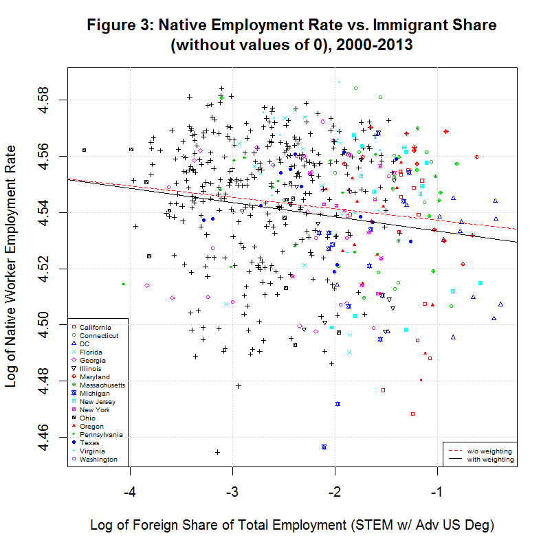
As before, the values being correlated appear as a relatively random cloud of values. Still, a regression line can be fit to any set of data. The red line is a simple regression of the natural log of the native worker employment rate versus the natural log of the foreign STEM share (with advanced U.S. degrees) of total employment. The black line is a regression using a weighting used by Zavodny in her study. Both lines again show a negative relation.
30. The Effect of Dummy or Indicator Variables on the Study
As mentioned above, following is the line in Zavodny's execution file that does the regression that we are trying to replicate:
xi: reg lnemprate_native lnimmshare_emp_stem_e_grad lnimmshare_emp_stem_n_grad i.statefip i.year [aw=weight_native] if year<2008, robust cluster(statefip)
As can be seen, the terms i.statefip and i.year appear among the arguments. These are dummy or indicator variables for the states and years, respectively. A short article titled "The Use of Dummy Variables in Regression Analysis" describes a dummy or indicator variable as "an artificial variable created to represent an attribute with two or more distinct categories/levels". Among things to keep in mind about dummy variables, it states that "the number of dummy variables necessary to represent a single attribute variable is equal to the number of levels (categories) in that variable minus one". For the eight years 2000 through 2007, seven dummy variables are required. Each of seven of the years will be indicated by having a unique one of the dummy variables set to one and the rest set to zero. The eighth year is the default and will be indicated if none of the seven indicators is set. Similarly, the 50 states plus D.C. will require 50 dummy variables.
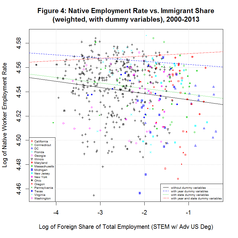
The following plot shows the effect of using the state and/or year dummy variables in the weighted regression:
In addition, following table shows the properties of the four regression lines:
[1] "                          CORREL                                              "
[1] " N  INTERCEPT    SLOPE     COEF   P-VALUE  DESCRIPTION                        "
[1] "--  ---------  --------  -------  -------  -----------------------------------"
[1] "2000-2013, WEIGHTED WITH DUMMY VARIABLES"
[1] " 5)    4.5281   -0.0051  -0.1308   0.0002  without dummy variables"
[1] " 6)    4.5598   -0.0026  -0.1308   0.0000  with year dummy variables only"
[1] " 7)    4.5336   -0.0046  -0.1308   0.0001  with state dummy variables only"
[1] " 8)    4.5734    0.0020  -0.1308   0.0000  with year and state dummy variables"
As can be seen, all of the regression lines have negative slopes except for the last one which uses both the year and state dummy variables. This is the red line in the plot.
In fact, the addition of these dummy variables may be appropriate. As can be seen in the graph of the Native Employment Rate vs. Year in California below, the native employment rate went down sharply in 2002 and 2003, just after the tech crash and the 2001 recession. The model may therefore benefit from having a variable based on year to account for such nationwide economic events. Similarly, the model may benefit from a variable based on the state because some states may have a lower base employment rate than other states. This was especially due when using the original questionable definition of the employment rate defined in the study. It effectively counted retired people as unemployed so that states with large retired populations (like Florida) likely had lower base employment rates.
However, just as the addition of dummy variables to account for the year and state may improve the model, so might the addition of others. The study's model is essentially stating that all changes in the native employment rate that are not due to the year or state are due to the number of foreign-born students with an advanced degree from a U.S. university who stays to work in a STEM field. But how about other foreign-born workers? Elsewhere in the study, it suggests that these workers also create jobs. It would appear that both sets of workers may essentially be given credit for creating the same job. At the very least, it would be instructive to test a model in which all of those workers were variables in the same model.
31. Removing the Effects of Year and State from the Scatter Plot
Regression 8 above is based on a weighted regression with three independent variables (immigrant share, year, and state). It is theoretically possible that the apparent lack of correlation in the scatter plot in Figure 4 is due to the year and/or state and not immigrant share (of STEM workers with advanced US degrees). In fact, it is possible to remove the predicted effects of the year and state from the scatter plot by doing an unweighted regression with the three variables. That regression is shown as regression 9 in the following table:
[1] "                          CORREL                                              "
[1] " N  INTERCEPT    SLOPE     COEF   P-VALUE  DESCRIPTION                        "
[1] "--  ---------  --------  -------  -------  -----------------------------------"
[1] "2000-2013, NATIVE WORKER EMPLOYMENT RATE ADJUSTED TO REMOVE EFFECTS OF YEAR AND STATE"
[1] " 9)    4.5681   0.00155  -0.1308   0.0000  with year and state dummy variables, unweighted"
[1] "10)    4.5681   0.00155   0.1307   0.0020  native employment rate adjusted to remove effects of year and state"
[1] "11)    4.5679   0.00145   0.1307   0.0038  native employment rate adjusted to remove effects of year and state, weighted"
Passing the result of this regression to the summary function gives coefficients for the following formula:
y = c1*im + c2*y1 + c3*y2 + ... + c8*y8 + c9*s2 + c10*s3 + ... + c58*s51

where y  = predicted log of native employment rate
      cN = coefficients
      im = log of immigrant share (of STEM workers with advanced US degrees)
      yN = 1 if data point is for year N, otherwise set to 0
      sN = 1 if data point is for state N, otherwise set to 0
The predicted effect of the year and state can then be removed by subtracting all but the first term (c1*im) in the above equation from the y-values in the scatter plot. That results in the following plot:
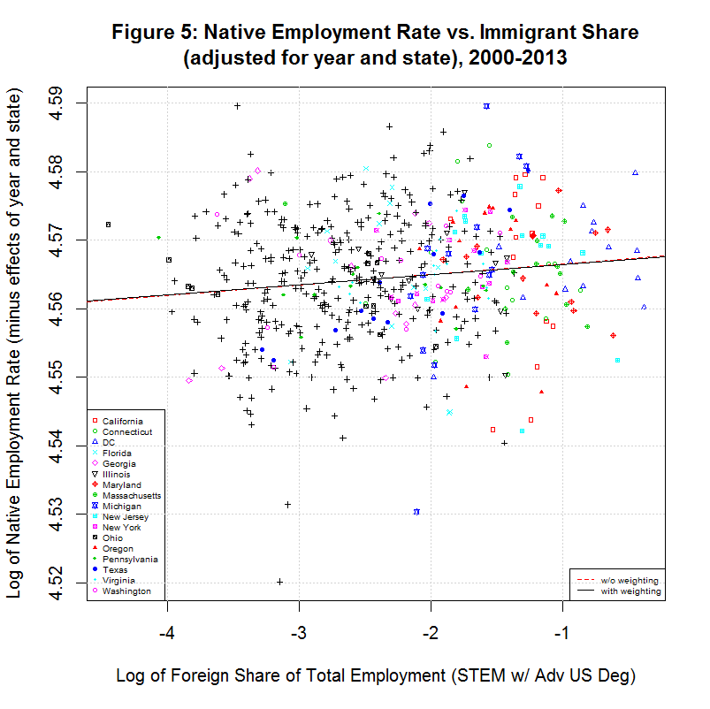
The red and black lines are the unweighted and weighted regression lines based on the adjusted data. Their coefficients are shown in regressions 10 and 11 in the table above. Note that the unweighted regression (10) has the exact same intercept and slope as the multivariable regression (9). This indicates that the adjustment was done correctly. The correlation coefficient is different because the data has been adjusted, backing out the predicted effect of the year and state. Both the low value of the correlation coefficient and the visible appearance of the adjusted data show that there is little correlation between the native employment rate and the immigrant share, even after accounting for the year and state.
32. Removing the Effects of Year from the Scatter Plot
Because of the lack of correlation, it would be instructive to look at some of the key states individually. It would still seem advisable to remove the apparent effect of the year. We can repeat the process of the prior section but apply it to just the year, not the year and state, by doing an unweighted regression with the immigrant share and the year. That regression is shown as regression 12 in the following table:
[1] "                          CORREL                                              "
[1] " N  INTERCEPT    SLOPE     COEF   P-VALUE  DESCRIPTION                        "
[1] "--  ---------  --------  -------  -------  -----------------------------------"
[1] "2000-2013, NATIVE WORKER EMPLOYMENT RATE ADJUSTED TO REMOVE EFFECTS OF YEAR ONLY"
[1] "12)    4.5583  -0.00300  -0.1308   0.0000  with year dummy variable, unweighted"
[1] "13)    4.5583  -0.00300  -0.1544   0.0003  native employment rate adjusted to remove effects of year"
[1] "14)    4.5555  -0.00288  -0.1544   0.0001  native employment rate adjusted to remove effects of year, weighted"
Passing the result of this regression to the summary function gives coefficients for the following formula:
y = c1*im + c2*y1 + c3*y2 + ... + c8*y8

where y  = predicted log of native employment rate
      cN = coefficients
      im = log of immigrant share (of STEM workers with advanced US degrees)
      yN = 1 if data point is for year N, otherwise set to 0
The predicted effect of the year can then be removed by subtracting all but the first term (c1*im) in the above equation from the y-values in the scatter plot. That results in the following plot:
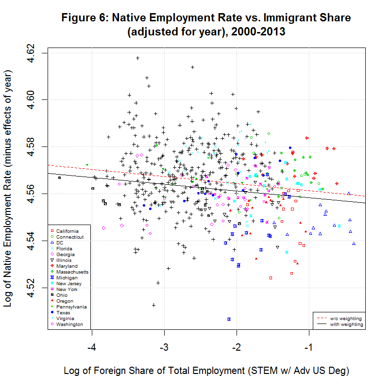
The red and black lines are the unweighted and weighted regression lines based on the adjusted data. Their coefficients are shown in regressions 13 and 14 in the table above. As before, note that the unweighted regression (13) has the exact same intercept and slope as the multivariable regression (12). This indicates that the adjustment was done correctly.
Because the data is no longer adjusted for state, it's now possible to see the difference between the base native employment rate of some of the key states. As can be seen, California and Oregon have among the lowest and Maryland is among the highest. Also of note is that the slope of both the weighted and unweighted regression lines are now negative, countering the key finding of the study. To get a better idea of what is going on, however, it's useful to look at the individual states.
33. Looking at the States Individually
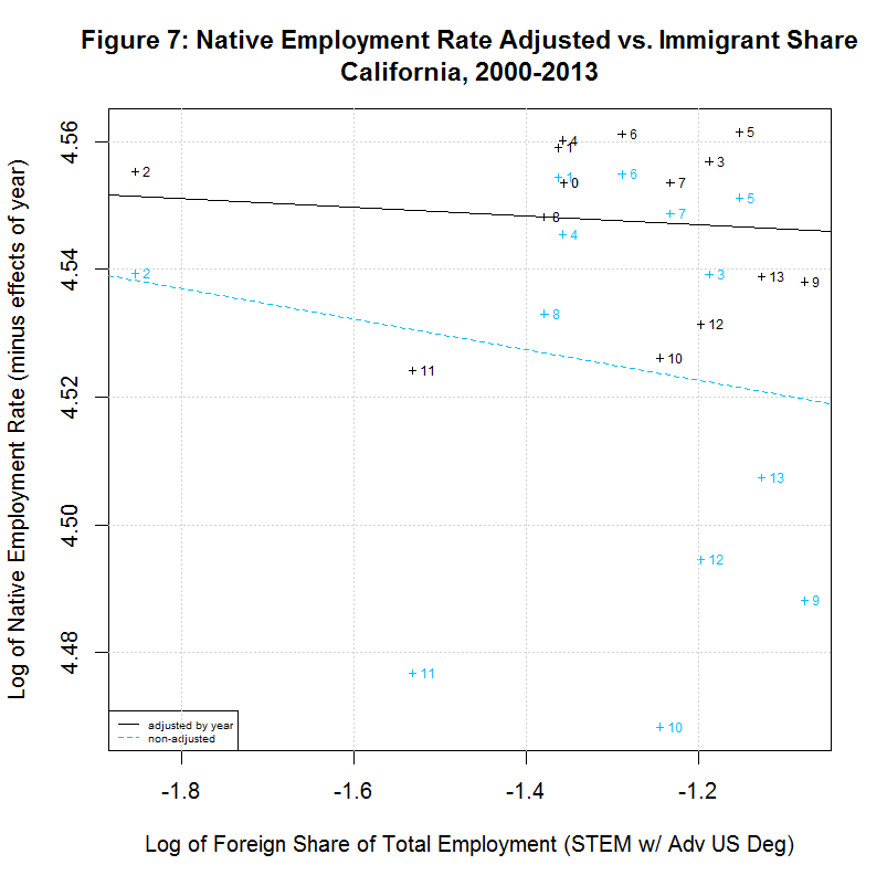
The following table shows the results of regressions for each of the 17 states listed in the legends of the previous plots. It uses the year-adjusted data obtained in the previous section. These 17 states include the 16 states that had the largest number of foreign-born STEM workers with advanced US degrees from 2000 to 2007. They also include the District of Columbia since it had the largest share of such workers as a percentage of total employment.
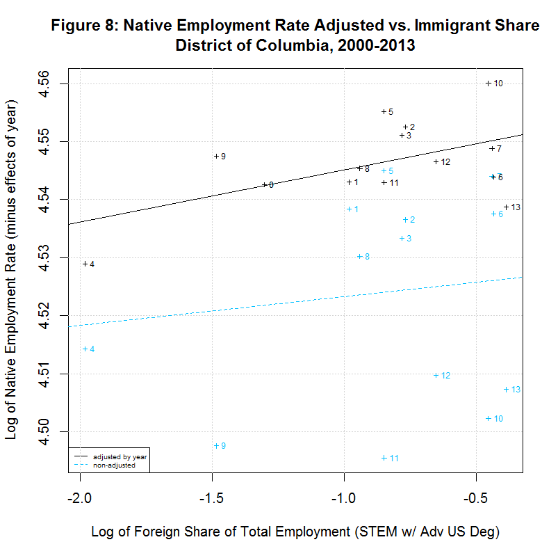
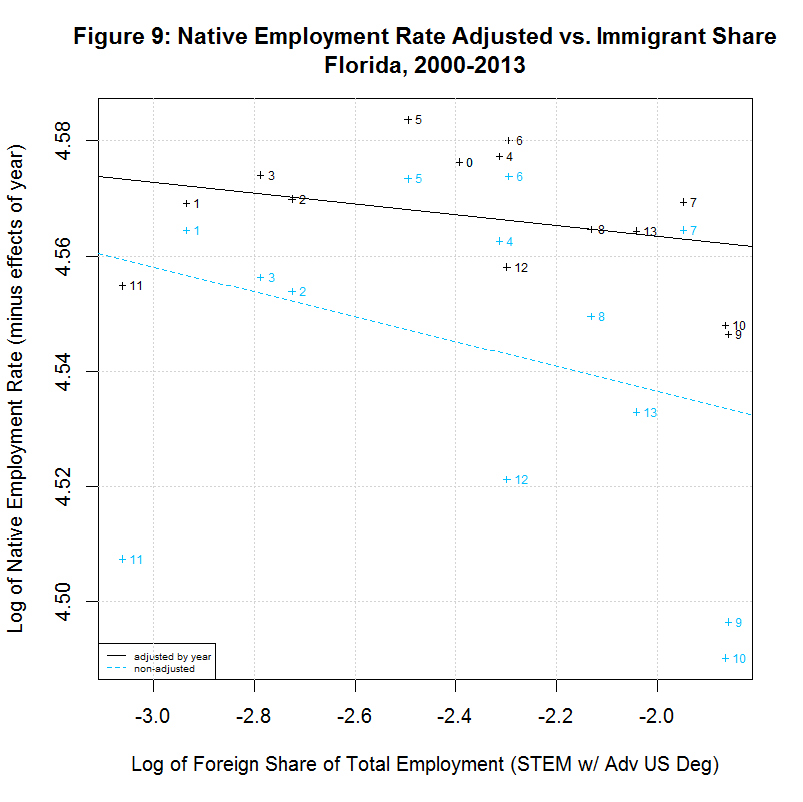
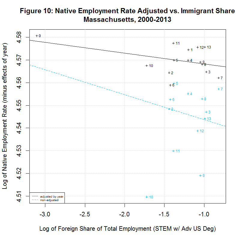
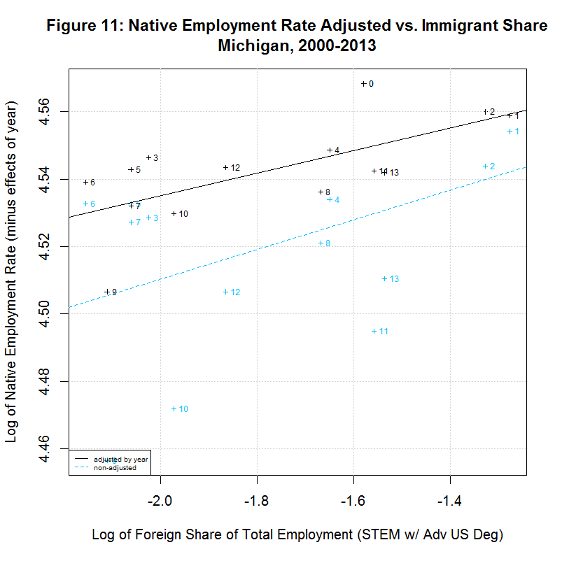
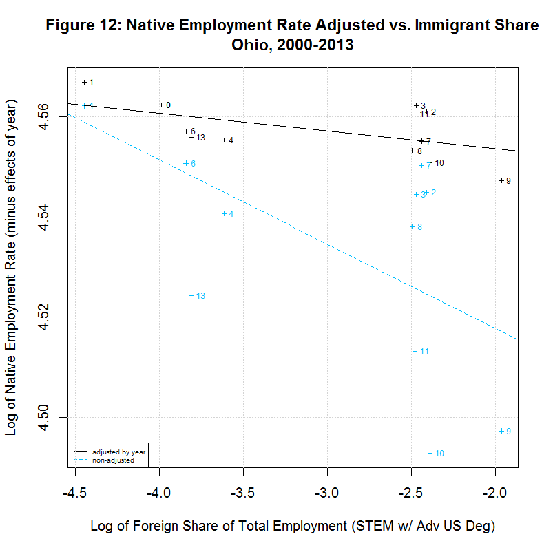
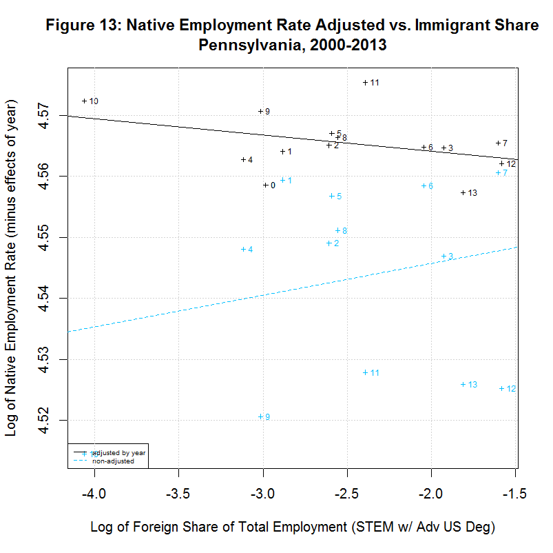
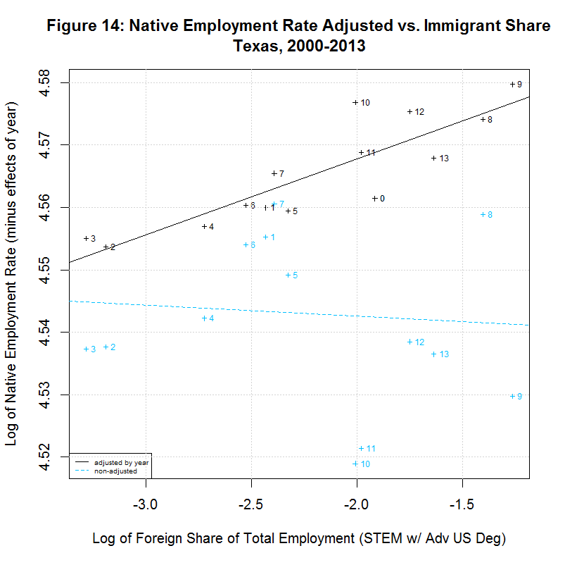
[1] "                          CORREL                                              "
[1] " N  INTERCEPT    SLOPE     COEF   P-VALUE  DESCRIPTION                        "
[1] "--  ---------  --------  -------  -------  -----------------------------------"
[1] "2000-2013, NATIVE WORKER EMPLOYMENT RATE (YEAR-ADJUSTED) VS IMMIGRANT SHARE, BY STATE"
[1] "15)    4.5387   -0.0069  -0.1021   0.7285  California"
[1] "16)    4.5641   -0.0017  -0.0729   0.8044  Connecticut"
[1] "17)    4.5541    0.0090   0.5385   0.0469  District of Columbia"
[1] "18)    4.5447   -0.0094  -0.3175   0.2687  Florida"
[1] "19)    4.5653    0.0017   0.0992   0.7471  Georgia"
[1] "20)    4.5468   -0.0031  -0.2121   0.4867  Illinois"
[1] "21)    4.5725   -0.0011  -0.0752   0.7983  Maryland"
[1] "22)    4.5635   -0.0048  -0.4285   0.1264  Massachusetts"
[1] "23)    4.6022    0.0336   0.6688   0.0089  Michigan"
[1] "24)    4.5536   -0.0051  -0.2032   0.4859  New Jersey"
[1] "25)    4.5643    0.0013   0.0648   0.8258  New York"
[1] "26)    4.5466   -0.0035  -0.5361   0.0724  Ohio"
[1] "27)    4.5414   -0.0049  -0.1633   0.5769  Oregon"
[1] "28)    4.5588   -0.0027  -0.3750   0.1864  Pennsylvania"
[1] "29)    4.5921    0.0122   0.8692   0.0001  Texas"
[1] "30)    4.5862    0.0025   0.2292   0.4307  Virginia"
[1] "31)    4.5610    0.0023   0.2442   0.4213  Washington"
As can be seen, 10 of the states had negative slopes (and correlation coefficients) and 7 had positive slopes. This is reverse the 7 negative and 10 positive slopes for 2000 to 2007. In any case, 7 had correlation cofficients above 0.37 and the plots of these 7 are shown in Figures 8 to 14 at the bottom of this page. Also shown is California which had the largest number of such workers. California seems especially important to look at since it had nearly three times the number of such workers as the next highest state, New York, and over a quarter of the total in the United States.
All of the plots contain the data and regression line for the year-adjusted data in black and the non-adjusted data in blue. The numbers next to the data indicate the year with 0 to 13 indicating 2000 to 2013. The data point for 2000 is identical for both sets of data because 2000 is the base year. For all other years, the adjusted numbers are higher than the unadjusted numbers. This adjustment generally increases through 2003, then decreases through 2007, increases again sharply through 2010, and then decreases somewhat through 2013. The increases in the adjustment in 2000 through 2003 and in 2007 through 2010 are likely adjusting for the large drop in the native employment rate during and after the 2001 and 2008 recessions.
As can be seen in the plot for California, there is a negative slope to the regression line, countering the key finding of the study. Also, the labels show that the native employment rate was generally dropping in California from 2007 through 2011 with a partial recovery after that. The same negative slope can be seen in Florida, Massachusetts, Ohio, and Pennsylvania. On the other hand, the District of Columbia, Michigan, and Texas have positive slopes.
As before, Michigan is interesting in that, despite the positive slope, both variables generally decreased from 2001 through 2006. There has since been a partial recovery through 2013. Texas is interesting in that it has the highest correlation at 0.87 but that also consists of both variables moving together in both directions. They both moved down from 2000 to 2002, then up from 2003 through 2009, and then they both backed off some through 2013.
Looking at the individual states shows that, whatever correlation there may or may not be on the national level, there is often a very different situation in key states. Any such correlation is of little help to workers in California where over a quarter of such workers are located. In addition, when both variables are shrinking, it seems very unlikely that a positive correlation reveals anything about how the growth of one variable will affect the other.
The R summary function provides a number of statistics for any regression. Among those included are the Multiple R-Squared, Adjusted R-Squared, F-Statistic, and p-value. Following are those statistics for the regressions in this analysis:
[1] "     MULTIPLE   ADJUSTED      F-                                    "
[1] " N  R-SQUARED  R-SQUARED  STATISTIC  DF1/DF2   P-VALUE   DESCRIPTION"
[1] "--  ---------  ---------  ---------  -------  ---------  -----------"
[1] "2000-2013, ALL DATA"
[1] " 1)    0.0233     0.0219    16.9813    1/712  4.219e-05  emprate_native ~ immshare_emp_stem_e_grad"
[1] "2000-2013, EXCLUDING POINTS WITH ZERO FOREIGN WORKERS IN STEM WITH ADVANCED US DEGREES"
[1] " 2)    0.0225     0.0208    12.7753    1/554  3.819e-04  emprate_native ~ immshare_emp_stem_e_grad"
[2] " 3)    0.0171     0.0153     9.6490    1/554  1.992e-03  lnemprate_native ~ lnimmshare_emp_stem_e_grad"
[3] " 4)    0.0247     0.0230    14.0470    1/554  1.970e-04  lnemprate_native ~ lnimmshare_emp_stem_e_grad, weights=weight_native"
[1] "2000-2013, WEIGHTED WITH DUMMY VARIABLES"
[1] " 5)    0.0247     0.0230    14.0470    1/554  1.970e-04  without dummy variables"
[2] " 6)    0.7113     0.7038    95.1879   14/541  2.658e-11  with year dummy variables only"
[3] " 7)    0.1827     0.1000     2.2090   51/504  1.070e-04  with state dummy variables only"
[4] " 8)    0.8743     0.8585    55.3070   62/493  5.215e-21  with year and state dummy variables"
[1] "2000-2013, NATIVE WORKER EMPLOYMENT RATE ADJUSTED TO REMOVE EFFECTS OF YEAR AND STATE"
[1] " 9)    0.8537     0.8346    44.7718   64/491  1.737e-13  with year and state dummy variables, unweighted"
[2] "10)    0.0171     0.0153     9.6311    1/554  2.011e-03  native employment rate adjusted to remove effects of year and state"
[3] "11)    0.0150     0.0132     8.4338    1/554  3.830e-03  native employment rate adjusted to remove effects of year and state, weighted"
[1] "2000-2013, NATIVE WORKER EMPLOYMENT RATE ADJUSTED TO REMOVE EFFECTS OF YEAR ONLY"
[1] "12)    0.6108     0.6008    60.6509   14/541  1.410e-06  with year dummy variable, unweighted"
[2] "13)    0.0238     0.0221    13.5230    1/554  2.586e-04  native employment rate adjusted to remove effects of year"
[3] "14)    0.0260     0.0243    14.8164    1/554  1.323e-04  native employment rate adjusted to remove effects of year, weighted"
[1] ""
[1] "      MULTIPLE   ADJUSTED      F-                                    "
[1] "  N  R-SQUARED  R-SQUARED  STATISTIC  DF1/DF2   P-VALUE   DESCRIPTION"
[1] "---  ---------  ---------  ---------  -------  ---------  -----------"
[1] "2000-2013, NATIVE WORKER EMPLOYMENT RATE (YEAR-ADJUSTED) VS IMMIGRANT SHARE, BY STATE"
 [1] "15)    0.0104    -0.0720     0.1263    1/ 12  7.285e-01  California"
 [2] "16)    0.0053    -0.0776     0.0641    1/ 12  8.044e-01  Connecticut"
 [3] "17)    0.2900     0.2308     4.9016    1/ 12  4.695e-02  District of Columbia"
 [4] "18)    0.1008     0.0259     1.3450    1/ 12  2.687e-01  Florida"
 [5] "19)    0.0098    -0.0802     0.1094    1/ 11  7.471e-01  Georgia"
 [6] "20)    0.0450    -0.0418     0.5180    1/ 11  4.867e-01  Illinois"
 [7] "21)    0.0057    -0.0772     0.0683    1/ 12  7.983e-01  Maryland"
 [8] "22)    0.1836     0.1155     2.6984    1/ 12  1.264e-01  Massachusetts"
 [9] "23)    0.4473     0.4012     9.7116    1/ 12  8.915e-03  Michigan"
[10] "24)    0.0413    -0.0386     0.5169    1/ 12  4.859e-01  New Jersey"
[11] "25)    0.0042    -0.0788     0.0506    1/ 12  8.258e-01  New York"
[12] "26)    0.2874     0.2161     4.0330    1/ 10  7.239e-02  Ohio"
[13] "27)    0.0267    -0.0544     0.3290    1/ 12  5.769e-01  Oregon"
[14] "28)    0.1406     0.0690     1.9639    1/ 12  1.864e-01  Pennsylvania"
[15] "29)    0.7556     0.7352    37.0943    1/ 12  5.414e-05  Texas"
[16] "30)    0.0525    -0.0264     0.6651    1/ 12  4.307e-01  Virginia"
[17] "31)    0.0596    -0.0258     0.6977    1/ 11  4.213e-01  Washington"
[1] ""
[1] "     MULTIPLE   ADJUSTED      F-                                    "
[1] " N  R-SQUARED  R-SQUARED  STATISTIC  DF1/DF2   P-VALUE   DESCRIPTION"
[1] "--  ---------  ---------  ---------  -------  ---------  -----------"
[1] "2000-2013, OLS WITH YEAR, STATE, AND SPECIFIED GROUP OF FOREIGN WORKERS"
[1] "32)    0.8750     0.8587    53.6851   64/491  5.038e-21  Advanced US degree and in STEM occupation"
[2] "33)    0.8661     0.8505    55.3869   64/548  5.832e-08  Advanced foreign degree and in STEM occupation"
[3] "34)    0.8755     0.8577    49.4266   64/450  1.157e-19  Advanced US|foreign degree and in STEM occupation"
[4] "35)    0.8661     0.8515    59.5258   64/589  5.387e-15  Advanced degree and in STEM occupation"
[5] "36)    0.8621     0.8485    63.2902   64/648  2.746e-38  Advanced degree"
[6] "20)    0.8620     0.8484    63.3686   64/649  5.604e-35  Bachelor's degree or higher"
[7] "38)    0.8622     0.8485    63.2279   64/647  7.518e-40  Advanced degree and NOT in STEM occupation"
[8] "39)    0.8620     0.8484    63.3522   64/649  5.464e-30  Bachelor's degree only"
[1] "2000-2013, OLS WITH YEAR, STATE, AND 4 SUBSETS OF FOREIGN WORKERS WITH BACHELOR'S DEGREE OR HIGHER"
[1] "40)    0.8756     0.8572    47.6662   66/447  1.376e-19  OLS with Year, State, and 4 Subsets"
Since the data includes the original 2000 to 2007 period, the conclusions that applied to that period generally apply to this period as well. After updating the data through 2013 and using an arguably better measure of the native worker employment rate, all of the regressions showed a negative correlation between the native worker employment rate and the share of total employment of foreign stem workers with advanced U.S. degrees except for the specific model on which the 262 number is based. For this model, the slope of the regression decreased from 0.0042 to 0.0020. Since the 262 number was based on a slope of 0.0040, this would halve the estimate. Of course, the negative correlation is weak and correlation does not mean causation.
This analysis has convinced me that any study that is to be used to shape public policy should be required to supply, not just the sources and methods by which its conclusions were reached, but also an environment in which such conclusions can be duplicated and the methods for reaching them can be examined and modified. For simple calculations, a spreadsheet and a process for extracting it from the original data source might be sufficient. But for more complex calculations such as were done here, the study should be required to supply the programs for both extracting and for processing the data. To that end, you can find links to all of the programs which I used in this analysis at this link. They all use the language R, described here as a free software environment for statistical computing and graphics.