A study titled "STEM Workers, H-1B Visas, and Productivity in US Cities", written by economist Giovanni Peri, Kevin Shih, and Chad Sparber, was released by the Journal of Labor Economics on July 1, 2015. Following is the last paragraph of the study's conclusion:
We find that a 1 percentage point increase in the foreign STEM share of a city's total employment increased the wage growth of native college-educated labor by about 7-8 percentage points and the wage growth of non-college-educated natives by 3-4 percentage points. We find insignificant effects on the employment of those two groups. These results indicate that STEM workers spur economic growth by increasing productivity, especially that of college-educated workers.
That is almost identical to the last paragraph of the version of the paper at this link except that it omits the following final sentence:
They also experienced increasing housing rents, which eroded part of their wage gain.
In any case, the study contains the following numbers in the first row of Table 5:
Table 5: The Effects of Foreign STEM on Native Wages and Employment

                       Weekly Wage,  Weekly Wage,    Weekly Wage,        Employment,  Employment,     Employment,
Explanatory Variable:  Native STEM   Native College  Native Non-College  Native STEM  Native College  Native Non-College
Growth Rate of                       educated        educated                         educated        educated
Foreign–STEM                (1)            (2)            (3)                 (4)            (5)            (6)
---------------------  ------------  --------------  ------------------  -----------  --------------  ------------------
(a) Baseline 2SLS;         6.65           8.03***        3.78**              0.53           2.48           5.17
O*NET 4% Definition       (4.53)         (3.03)         (1.75)              (0.56)         (4.69)         (4.20)

  * Significant at the 10% level.
 ** Significant at the 5% level.
*** Significant at the 1% level.
These are almost identical to the numbers in Table 6 at the aforementioned link. One big difference is that the top number (the slope) for the last column is 5.17 in the paper but -5.17 in the link. In fact, Giovanni Peri sent me a 30 April, 2014 version of this paper in which the value was likewise -5.17. Hence, it appears that this was an error in the study, at least in the initial Journal of Labor Statistics version.
Replication of Six Key Findings Using Study's Data and Shiny
Following are the statements that generate the 6 regressions from which the values in the first row of Table 5 are derived. They are taken from the file Table_5_April_30_2014.do:
*Table 5, row (a)
* explanatory is STEM O*net definition 4%, coefficients (1)-(6) in order
xi: ivreg2 delta_native_stemO4_wkwage (delta_imm_stemO4 = delta_imm_stemO4_H1B_hat80) bartik_coll_wage bartik_coll_emp i.year i.metarea if year>1990 & panel1980==1, robust cluster(metarea)
test delta_imm_stemO4==8.03
xi: ivreg2 delta_native_coll_wkwage (delta_imm_stemO4 = delta_imm_stemO4_H1B_hat80) bartik_coll_wage bartik_coll_emp i.year i.metarea if year>1990 & panel1980==1, robust cluster(metarea)
xi: ivreg2 delta_native_nocoll_wkwage (delta_imm_stemO4 = delta_imm_stemO4_H1B_hat80) bartik_nocoll_wage bartik_nocoll_emp i.year i.metarea if year>1990 & panel1980==1, robust cluster(metarea)
xi: ivreg2 delta_native_stemO4_emp (delta_imm_stemO4 = delta_imm_stemO4_H1B_hat80) bartik_coll_wage bartik_coll_emp i.year i.metarea if year>1990 & panel1980==1, robust cluster(metarea)
xi: ivreg2 delta_native_coll_emp (delta_imm_stemO4 = delta_imm_stemO4_H1B_hat80) bartik_coll_wage bartik_coll_emp i.year i.metarea if year>1990 & panel1980==1, robust cluster(metarea)
xi: ivreg2 delta_native_nocoll_emp (delta_imm_stemO4 = delta_imm_stemO4_H1B_hat80) bartik_nocoll_wage bartik_nocoll_emp i.year i.metarea if year>1990 & panel1980==1, robust cluster(metarea)
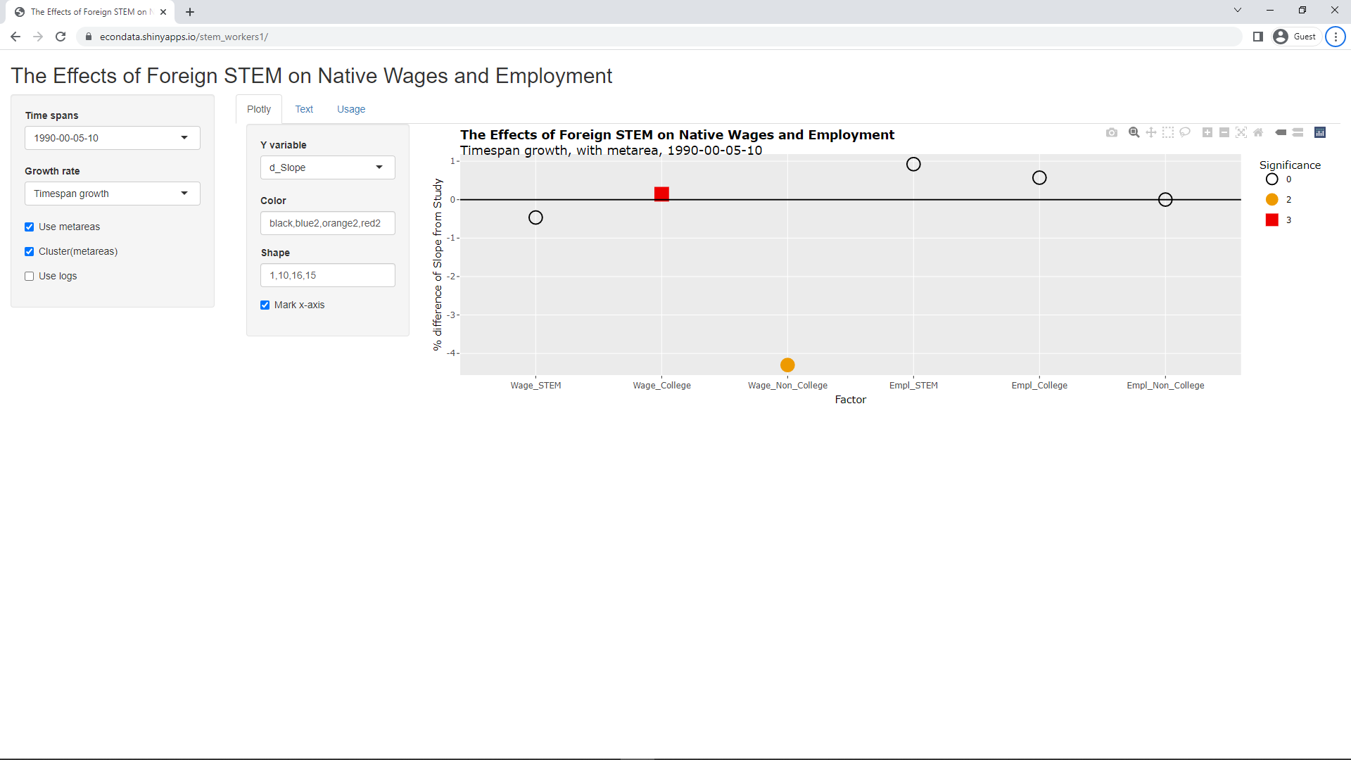
An attempt to replicate the six key slopes in row 1 of Table 5 was made in the R language using the ivreg function in the ivreg package. Also, to replicate the "robust cluster(metarea)" specification at the end of the Stata code above, it was necessary to use the sandwich package and the lmtest package as described in Option 1 at this link. The R code to replicate the key findings was used to create a dashboard using a framework called Shiny which can be used to see the effects of the various options used in the study. The code for this Shiny app can be found at this link and a running version of it can be accessed at https://econdata.shinyapps.io/stem_workers1/. When run, the following initial screen is displayed:
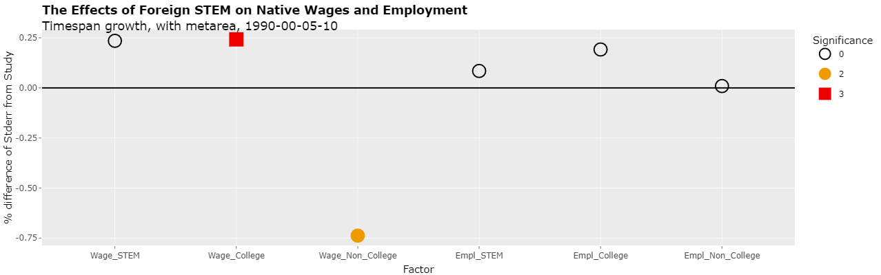
The plot shows the percent difference between the slopes of the reproduce regressions with the slopes of the regressions as reported in the study. Changing the select list "Y variable" to "d_Stderr" will show the same information (percent difference) for the standard errors:
Clicking on the Text tab will display the following actual numbers:
Table 5 - The Effects of Foreign STEM on Native Wages and Employment

Timespan growth, with metarea, 1990-00-05-10

    CALCULATED VALUES                                    STUDY VALUES          % DIFFERENCES   DIFF
    ---------------------------------------------------  -------------------  ---------------- ----
 N  INTERCEPT     SLOPE   STDERR   TVALUE   PVALUE  SIG   SLOPE  STDERR  SIG    SLOPE   STDERR  SIG  DESCRIPTION
--  ---------  --------  -------  -------  -------  ---  ------  ------  ---  -------  -------  ---  -----------
 1    -0.3322    6.6191    4.541    1.458    0.146    0    6.65    4.53    0   -0.464    0.235    0  Weekly Wage, Native STEM
 2    -0.0764    8.0414    3.037    2.648    0.008    3    8.03    3.03    3    0.142    0.242    0  Weekly Wage, Native College-Educated
 3     0.0594    3.6174    1.737    2.082    0.038    2    3.78    1.75    2   -4.302   -0.737    0  Weekly Wage, Native Non-College-Educated
 4     0.0272    0.5349    0.560    0.954    0.340    0    0.53    0.56    0    0.924    0.085    0  Employment, Native STEM
 5     0.0311    2.4942    4.699    0.531    0.596    0    2.48    4.69    0    0.572    0.192    0  Employment, Native College-Educated
 6    -0.2557   -5.1701    4.200   -1.231    0.219    0   -5.17    4.20    0    0.002    0.009    0  Employment, Native Non-College-Educated
As can be seen from the "% DIFFERENCES" columns, all of the reproduced slopes are within one percent of the slopes given in the study except for "Weekly Wage, Native Non-College-Educated" which differs by just 4.3 percent. All of the reproduced standard errors are within an even closer 0.25 percent except for the same "Weekly Wage, Native Non-College-Educated" which differs by less than 0.75 percent. The "DIFF" column shows that the significance numbers did not differ with those in the study. The reason for the single 4.3 percent difference in slope is not clear. It would seem that it could be a difference between Stata's ivreg2 and R's ivreg methods but it could also be a minor reporting error in the study as when the sign was incorrectly dropped for "Employment, Native Non-College-Educated". In any case, even the 4.3 percent is a very small difference.
Still, these minor differences show a problem with the fact that many of these studies are generated using Stata which, according to prices at this link, is $840 per year for a Business single-user. According to this link, Stata is used by many researchers but it seems likely that most individuals use the free languages of R and/or Python. It would seem reasonable for all findings from studies that are used to set public policy be required to be reproducible in a free publicly available language like R or Python. Using a costly language like Stata puts an unnecessary burden on those who reproduce the study, even if the code is made available. Besides obscuring the cause of any differences, additional effort was required to convert Stata code to R. For example, as previously described, additional packages and efforts were required to replicate the "robust cluster(metarea)" option in the Stata ivreg2 package.
Clicking on the Plotly tab and changing the select list "Y variable" to "Pvalue" will show the actual p-values of the 6 regressions as following:
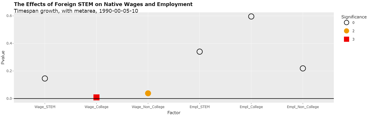
As can be seen, the 2nd regression is significant at the 1% level (less than 0.01) and the 3rd regression is significant to the 5% (less than 0.05) level. This is the same as was reported in the study.
Changing the select list "Y variable" to "Slope" will show the actual slopes of the 6 regressions as follows:
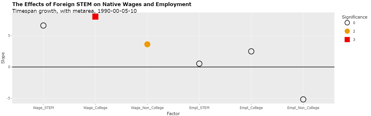
As can be seen, all of the slopes of the reproduced regressions are positive except for the last one. Interestingly, the minus sign of this last regression was omitted from the study.
The Use of Time Spans of Different Length
In fact, a close look at the data reveals a serious problem. As stated above, the three time spans are 1990-2000, 2000-2005, and 2005-2010. Hence, the first one is a 10-year span and the second and third are 5-year spans. As is likely the case with most readers of the study, I assumed that the different lengths were accounted for somehow, perhaps by using annualized growth figures. In fact, the figures are not annualized but are for the entire span. Following are the formulas for the dependent variables and instruments, taken from file Table_5_April_30_2014.do:
gen delta_native_stemO4_wkwage=(nat_stemO4_wkwage-nat_stemO4_wkwage[_n-1])/nat_stemO4_wkwage[_n-1] if year>=1980
gen delta_native_coll_wkwage=(nat_coll_wkwage-nat_coll_wkwage[_n-1])/nat_coll_wkwage[_n-1] if year>=1980
gen delta_native_nocoll_wkwage=(nat_nocoll_wkwage-nat_nocoll_wkwage[_n-1])/nat_nocoll_wkwage[_n-1] if year>=1980
gen delta_native_stemO4_emp=(nat_stemO4_emp-nat_stemO4_emp[_n-1])/labforce[_n-1] if year>=1980
gen delta_native_coll_emp=(nat_coll_emp-nat_coll_emp[_n-1])/labforce[_n-1] if year>=1980
gen delta_native_nocoll_emp=(nat_nocoll_emp-nat_nocoll_emp[_n-1])/labforce[_n-1] if year>=1980
gen delta_imm_stemO4=(imm_stemO4-imm_stemO4[_n-1])/labforce[_n-1] if year>=1980
gen delta_imm_stemO4_H1B_hat80=(imm_stemO4_H1B_hat80-imm_stemO4_H1B_hat80[_n-1])/labforce_hat80[_n-1] if year>=1990
gen bartik_coll_wage=(pred_coll_wkwage-pred_coll_wkwage[_n-1])/pred_coll_wkwage[_n-1] if year>1990
gen bartik_nocoll_wage=(pred_nocoll_wkwage-pred_nocoll_wkwage[_n-1])/pred_nocoll_wkwage[_n-1] if year>1990
gen bartik_coll_emp=(pred_coll_emp-pred_coll_emp[_n-1])/pred_emp[_n-1] if year>1990
gen bartik_nocoll_emp=(pred_nocoll_emp-pred_nocoll_emp[_n-1])/pred_emp[_n-1] if year>1990
Following are the same formulas with spacing added so that their similar structures and be compared:
gen delta_native_stemO4_wkwage=(nat_stemO4_wkwage   -nat_stemO4_wkwage[_n-1])   /nat_stemO4_wkwage[_n-1]  if year>=1980
gen delta_native_coll_wkwage  =(nat_coll_wkwage     -nat_coll_wkwage[_n-1])     /nat_coll_wkwage[_n-1]    if year>=1980
gen delta_native_nocoll_wkwage=(nat_nocoll_wkwage   -nat_nocoll_wkwage[_n-1])   /nat_nocoll_wkwage[_n-1]  if year>=1980
gen delta_native_stemO4_emp   =(nat_stemO4_emp      -nat_stemO4_emp[_n-1])      /labforce[_n-1]           if year>=1980
gen delta_native_coll_emp     =(nat_coll_emp        -nat_coll_emp[_n-1])        /labforce[_n-1]           if year>=1980
gen delta_native_nocoll_emp   =(nat_nocoll_emp      -nat_nocoll_emp[_n-1])      /labforce[_n-1]           if year>=1980
gen delta_imm_stemO4          =(imm_stemO4          -imm_stemO4[_n-1])          /labforce[_n-1]           if year>=1980
gen delta_imm_stemO4_H1B_hat80=(imm_stemO4_H1B_hat80-imm_stemO4_H1B_hat80[_n-1])/labforce_hat80[_n-1]     if year>=1990
gen bartik_coll_wage          =(pred_coll_wkwage    -pred_coll_wkwage[_n-1])    /pred_coll_wkwage[_n-1]   if year> 1990
gen bartik_nocoll_wage        =(pred_nocoll_wkwage  -pred_nocoll_wkwage[_n-1])  /pred_nocoll_wkwage[_n-1] if year> 1990
gen bartik_coll_emp           =(pred_coll_emp       -pred_coll_emp[_n-1])       /pred_emp[_n-1]           if year> 1990
gen bartik_nocoll_emp         =(pred_nocoll_emp     -pred_nocoll_emp[_n-1])     /pred_emp[_n-1]           if year> 1990
As can be seen, the formulas are comparing the values from successive time spans with no adjustment for the length of each span. To see the problem, consider the following short R program:
library("tidyverse")
label <- c("2005-2010","2000-2005","1990-2000")
span <- c(5,5,10) # number of units per span (units can be years, 5-years, etc.)
spanadj <- 0 # 0=no adj, 1=annualize, 5=adj to 5-year growth
npts <- 20 # number of points per span
xmean <- 1 # x mean per unit
xsd <- 1   # x stddev per unit
ymean <- 2 # y mean per unit
ysd <- 2   # y stddev per unit
seed1 <- 123 # initial seed for random numbers
set.seed(seed1)
xx <- NULL
yy <- NULL
ss <- NULL

for (i in 1:length(span)){
    for (j in 1:span[i]){
        if (j == 1){
            xx1 <- rnorm(npts, xmean, xsd)
            yy1 <- rnorm(npts, ymean, ysd)
        }
        else{
            xx2 <- rnorm(npts, xmean, xsd)
            yy2 <- rnorm(npts, ymean, ysd)
            xx1 <- ((((xx1/100)+1) * ((xx2/100)+1)) - 1) * 100
            yy1 <- ((((yy1/100)+1) * ((yy2/100)+1)) - 1) * 100
        }
    }
    if (spanadj > 0 & spanadj != span[i]){ # adjust growth rate
        xx1 <- (((xx1/100)+1) ^ (spanadj/span[i]) - 1) * 100
        yy1 <- (((yy1/100)+1) ^ (spanadj/span[i]) - 1) * 100
    }
    xx <- c(xx,xx1)
    yy <- c(yy,yy1)
    ss1 <- rep(label[i],length(xx1))
    ss <- c(ss,ss1)
}
dd <- data.frame(xx,yy,ss)
lm1 <- lm(yy ~ xx, data=dd)

gg <- ggplot(data=dd, aes(x=xx,y=yy)) +
    geom_point(aes(color=ss,shape=ss), size=3, alpha=1.0) +
    xlab("Percent Growth in STEM") + ylab("Percent Growth in Wage") +
    ggtitle(paste0("span=",paste0(span,collapse='|'),
                   ", xmn|xsd|ymn|ysd=",xmean,"|",xsd,"|",ymean,"|",ysd,
                   ", npts=",npts,", seed=",seed1, ", adj=",spanadj,
                   ", p-value=",format(summary(lm1)$coefficients[2,4],digits=4)))
print(gg)
print(summary(lm1))
This code does a simple simulation of data wherein the x variable grows at about 1 percent a year and the y variable grows at about 2 percent a year. More precisely, the growth each year in the x variable is taken from a random normal distribution with a mean of 1 and a standard deviation of 1. Similarly, the growth each year in the y variable is taken from a random normal distribution with a mean of 2 and a standard deviation of 2. This process is used to create 20 points for each of the spans, 1990-2000, 2000-2005, and 2005-2020. Starting with the seed 123 generates the following plot:
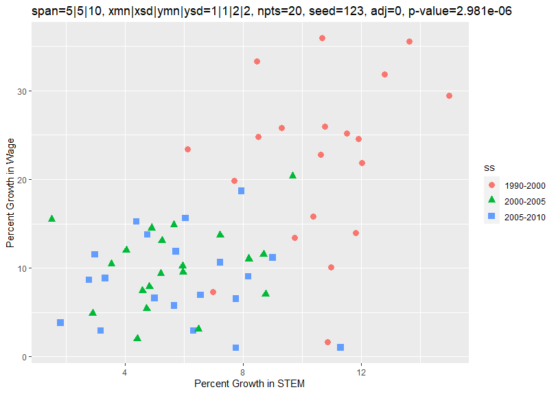
As can be seen, the growth of the data for 2000-2005 and 2005-2010 was about 5 and 10 percent on average along the x and y axes, about what you would expect since the annual growth rate was about 1 and 2 percent. However, the growth of the data for 1990-2000 was about 10 and 20 percent since the 1990-2000 time span was twice as long at 10 years. A regression on the x and y variables generated the following results:
Coefficients:
            Estimate Std. Error t value Pr(>|t|)
(Intercept)   1.9517     2.4569   0.794     0.43
xx            1.5950     0.3083   5.174 2.98e-06 ***
---
Signif. codes:  0 '***' 0.001 '**' 0.01 '*' 0.05 '.' 0.1 ' ' 1

Residual standard error: 7.449 on 58 degrees of freedom
Multiple R-squared:  0.3158,	Adjusted R-squared:  0.304
F-statistic: 26.77 on 1 and 58 DF,  p-value: 2.981e-06
This suggests that the x and y variables are closely correlated. However, the above program shows that there is no correlation between them except perhaps that both are generally increasing over time.
Changing spanadj from 0 to 1 and rerunning the program causes the growth rates to be annualized and generates the following plot:
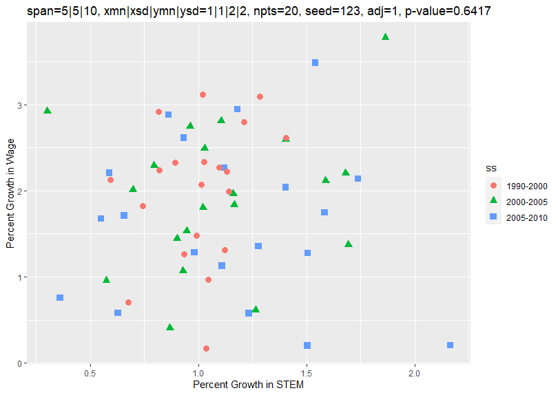
Now the growth rates of all 3 spans average about 1 and 2 percent along the x and y axes, what you would expect. A regression on the x and y variables now generates the following results:
Coefficients:
            Estimate Std. Error t value Pr(>|t|)
(Intercept)   1.7105     0.3477   4.919 7.53e-06 ***
xx            0.1424     0.3045   0.468    0.642
---
Signif. codes:  0 '***' 0.001 '**' 0.01 '*' 0.05 '.' 0.1 ' ' 1

Residual standard error: 0.8618 on 58 degrees of freedom
Multiple R-squared:  0.003757,	Adjusted R-squared:  -0.01342
F-statistic: 0.2188 on 1 and 58 DF,  p-value: 0.6417
The x and y variables now show no close correlation. This is as expected since they were generated independent of each other.
Changing spanadj to 5 and rerunning the program causes the growth rates to be adjusted to a 5-year growth rate and generates the following plot:
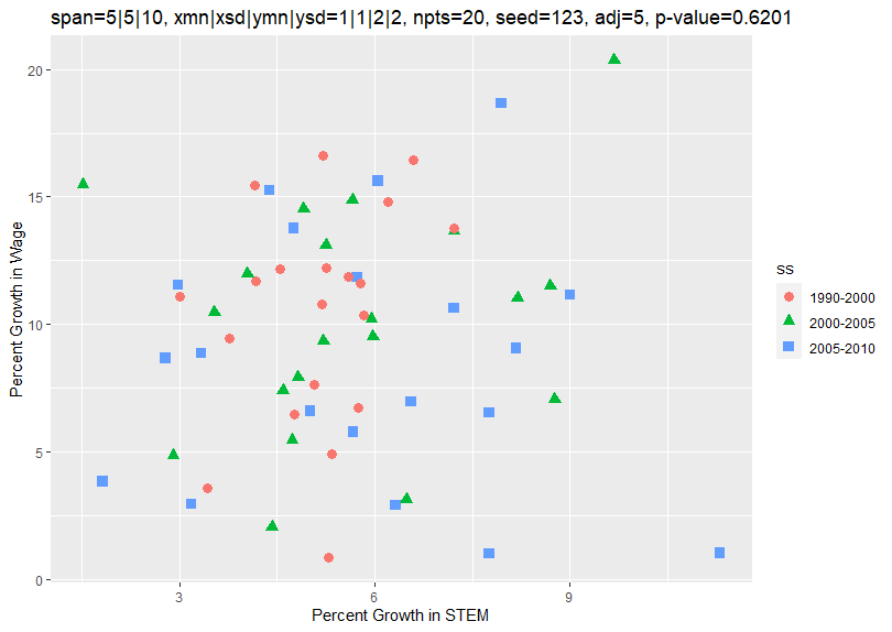
Now the growth rates of all 3 spans average about 5 and 10 percent along the x and y axes. This is what you would expect since the 1-year growth rate is about 1 and 2 percent. A regression on the x and y variables now generates the following results:
Coefficients:
            Estimate Std. Error t value Pr(>|t|)
(Intercept)   8.8909     1.8308   4.856 9.43e-06 ***
xx            0.1556     0.3123   0.498     0.62
---
Signif. codes:  0 '***' 0.001 '**' 0.01 '*' 0.05 '.' 0.1 ' ' 1

Residual standard error: 4.629 on 58 degrees of freedom
Multiple R-squared:  0.004264,	Adjusted R-squared:  -0.0129
F-statistic: 0.2483 on 1 and 58 DF,  p-value: 0.6201
Once again, the x and y variables now show no close correlation. As before, this is as expected since they were generated independent of each other.
The above program is a very simple simulation. But it does show that the use of time spans of different length can make there appear to be a correlation between the x and y variables when no such correlation should exist. The x and y variables are generated independently such that y is in no way a function of x. However, they are both a function of the time span. Since the formula does not account for the time span, it would seem that this is being misinterpreted as a correlation between the x and y variables. The program further shows that standardizing the growth rates, to 1-year or some other set time span, appears to avoid the problem.
Fixing the Problem of Differing Time Spans
This same principle shown with the simulated data applies to all of the regressions in Table 5 of the study. The time span 1990-2000 looks better in the growth of the x and y variables compared to the other time spans than is truly the case when taken on an annualized basis. The growth rates can be annualized in the Shiny application by changing the "Growth rate" select list from "Timespan growth" to "1-year growth". This results in the following plot:
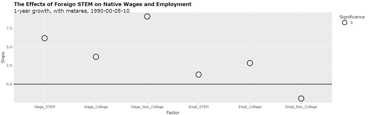
As can be seen, the slopes of the first 5 regressions are still positive. However, none of the regressions are now significant. Clicking on the Text tab shows the following:
Table 5 - The Effects of Foreign STEM on Native Wages and Employment

1-year growth, with metarea, 1990-00-05-10

    CALCULATED VALUES                                    STUDY VALUES          % DIFFERENCES   DIFF
    ---------------------------------------------------  -------------------  ---------------- ----
 N  INTERCEPT     SLOPE   STDERR   TVALUE   PVALUE  SIG   SLOPE  STDERR  SIG    SLOPE   STDERR  SIG  DESCRIPTION
--  ---------  --------  -------  -------  -------  ---  ------  ------  ---  -------  -------  ---  -----------
 1    -0.0188    6.2001   13.217    0.469    0.639    0    6.65    4.53    0   -6.765  191.776    0  Weekly Wage, Native STEM
 2    -0.0126    3.6896    8.554    0.431    0.666    0    8.03    3.03    3  -54.052  182.304   -3  Weekly Wage, Native College-Educated
 3     0.0131    9.1280    5.806    1.572    0.117    0    3.78    1.75    2  141.480  231.779   -2  Weekly Wage, Native Non-College-Educated
 4     0.0012    1.2894    0.960    1.343    0.180    0    0.53    0.56    0  143.274   71.470    0  Employment, Native STEM
 5     0.0029    2.8371    5.561    0.510    0.610    0    2.48    4.69    0   14.399   18.563    0  Employment, Native College-Educated
 6    -0.0071   -1.9430    6.210   -0.313    0.755    0   -5.17    4.20    0  -62.417   47.853    0  Employment, Native Non-College-Educated
As can be seen, the p-values are now range from 0.117 to 0.755 which is 11.7 to 75.5 percent.
The Use of Metropolitan Areas as a Dummy Variable
The indicator variable metarea is especially concerning. The data consists of values from 3 time spans (1990-2000, 2000-2005, and 2005-2010) taken from 219 metareas (metropolitan areas). In making metarea an indicator or dummy variable, 218 terms with 218 coefficients are added to the equation. In essence, each of the 219 metareas has its own independent coefficient based on a mere three data points. This arguably causes overfitting of the data.
An article on overfitting in regression models states the following:
Harrell describes a rule of thumb to avoid overfitting of a minimum of 10 observations per regression parameter in the model. Remember that each numerical predictor in the model adds a parameter. Each categorical predictor in the model adds k-1 parameters, where k is the number of categories.
The data consists of 657 values (from the 3 time spans and 219 metareas mentioned above). The use of a categorical variable for the 219 metropolitan areas results in 218 (k-1) parameters being added. That's about 3 observations per regression parameter (657/218) versus the minimum of 10 suggested in the rule of thumb above. That would certainly seem to raise the danger of overfitting.
The use of the metarea can be removed by unchecking the "Use metareas" checkbox. This results in the following plot:
As can be seen, the slopes of the last 4 regressions are now negative and 3 of them are with some level of significance. This would imply that foreign STEM have a NEGATIVE effect on the employment of native non-college educated workers with a significance at the 5% level! In addition, it would imply that foreign STEM have a negative effect on the weekly wage of those native non-college educated workers and the employment of native STEM workers with a significance at the 10% level.
Now, it would seem imprudent to immediately jump from the conclusion that foreign STEM have no effect on native workers to the conclusion that they have a serious effect based strictly on the use of metarea as an indicator variable. However, this would seem to very much support some of the principles put out by the American Statistical Association in 2016 in a paper titled "Statement on Statistical Significance and P-Values" which is described at this link. Perhaps most relevant in this case is the following 6th prinicple:
6. By itself, a p-value does not provide a good measure of evidence regarding a model or hypothesis.
Researchers should recognize that a p-value without context or other evidence provides limited information. For example, a p-value near 0.05 taken by itself offers only weak evidence against the null hypothesis. Likewise, a relatively large p-value does not imply evidence in favor of the null hypothesis; many other hypotheses may be equally or more consistent with the observed data. For these reasons, data analysis should not end with the calculation of a p-value when other approaches are appropriate and feasible.
Looking at Raw Growth Rates Versus the Natural Log of Growth Rates
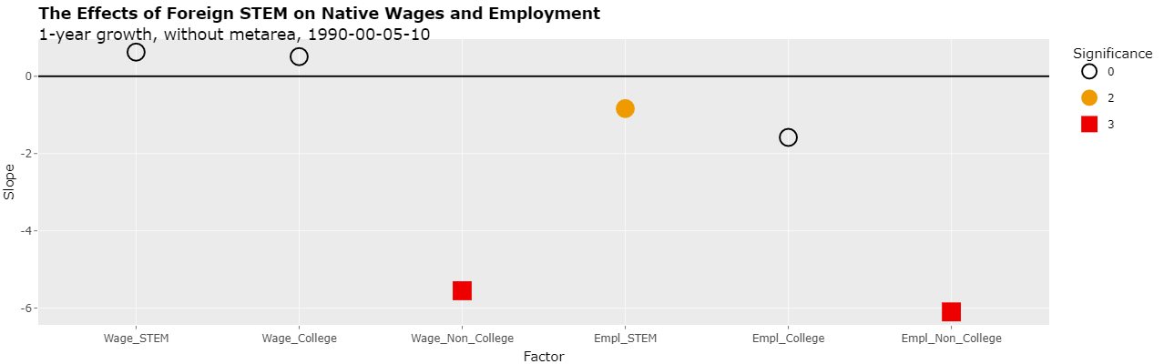
It should be noted that the use of time spans of different length described here appears very much to be a mistake and that the growth rates should be annualized or otherwise made properly comparable. Clicking on the Text tab will display the following:
Table 5 - The Effects of Foreign STEM on Native Wages and Employment

1-year growth, without metarea, 1990-00-05-10

    CALCULATED VALUES                                    STUDY VALUES          % DIFFERENCES   DIFF
    ---------------------------------------------------  -------------------  ---------------- ----
 N  INTERCEPT     SLOPE   STDERR   TVALUE   PVALUE  SIG   SLOPE  STDERR  SIG    SLOPE   STDERR  SIG  DESCRIPTION
--  ---------  --------  -------  -------  -------  ---  ------  ------  ---  -------  -------  ---  -----------
 1     0.0094    0.6247    3.715    0.168    0.867    0    6.65    4.53    0  -90.606  -17.997    0  Weekly Wage, Native STEM
 2    -0.0050    0.5081    2.707    0.188    0.851    0    8.03    3.03    3  -93.672  -10.669   -3  Weekly Wage, Native College-Educated
 3    -0.0058   -5.5511    1.716   -3.234    0.001    3    3.78    1.75    2 -246.855   -1.915    1  Weekly Wage, Native Non-College-Educated
 4     0.0030   -0.8367    0.342   -2.448    0.015    2    0.53    0.56    0 -257.873  -38.976    2  Employment, Native STEM
 5     0.0110   -1.5830    1.721   -0.920    0.358    0    2.48    4.69    0 -163.830  -63.315    0  Employment, Native College-Educated
 6    -0.0118   -6.0987    2.310   -2.641    0.008    3   -5.17    4.20    0   17.963  -45.009    3  Employment, Native Non-College-Educated
Now, simply changing the Growth rate select list to "5-year growth" will display the following:
Table 5 - The Effects of Foreign STEM on Native Wages and Employment

5-year growth, without metarea, 1990-00-05-10

    CALCULATED VALUES                                    STUDY VALUES          % DIFFERENCES   DIFF
    ---------------------------------------------------  -------------------  ---------------- ----
 N  INTERCEPT     SLOPE   STDERR   TVALUE   PVALUE  SIG   SLOPE  STDERR  SIG    SLOPE   STDERR  SIG  DESCRIPTION
--  ---------  --------  -------  -------  -------  ---  ------  ------  ---  -------  -------  ---  -----------
 1     0.0704   -8.7669    6.992   -1.254    0.210    0    6.65    4.53    0 -231.833   54.345    0  Weekly Wage, Native STEM
 2    -0.0152   -0.0694    2.767   -0.025    0.980    0    8.03    3.03    3 -100.865   -8.672   -3  Weekly Wage, Native College-Educated
 3    -0.0307   -5.5528    1.726   -3.217    0.001    3    3.78    1.75    2 -246.899   -1.372    1  Weekly Wage, Native Non-College-Educated
 4     0.0148   -0.8258    0.341   -2.420    0.016    2    0.53    0.56    0 -255.803  -39.069    2  Employment, Native STEM
 5     0.0536   -1.4843    1.841   -0.806    0.420    0    2.48    4.69    0 -159.852  -60.745    0  Employment, Native College-Educated
 6    -0.0589   -6.3830    2.473   -2.581    0.010    2   -5.17    4.20    0   23.461  -41.125    2  Employment, Native Non-College-Educated
Note that all of the numbers have changed except for STUDY even though we've only changed the length of the growth rate to which the data has been standardized. The problem is that, as explained at this link, one should use the logarithm of a growth rate in order to use a linear regression.
Checking the "Use logs" checkbox will return the following numbers for a 1-year growth rate:
Table 5 - The Effects of Foreign STEM on Native Wages and Employment

Log of 1-year growth, without metarea, 1990-00-05-10

    CALCULATED VALUES                                    STUDY VALUES          % DIFFERENCES   DIFF
    ---------------------------------------------------  -------------------  ---------------- ----
 N  INTERCEPT     SLOPE   STDERR   TVALUE   PVALUE  SIG   SLOPE  STDERR  SIG    SLOPE   STDERR  SIG  DESCRIPTION
--  ---------  --------  -------  -------  -------  ---  ------  ------  ---  -------  -------  ---  -----------
 1     0.0085    2.7673    3.524    0.785    0.433    0    6.65    4.53    0  -58.387  -22.204    0  Weekly Wage, Native STEM
 2    -0.0056    0.6451    2.756    0.234    0.815    0    8.03    3.03    3  -91.966   -9.036   -3  Weekly Wage, Native College-Educated
 3    -0.0057   -5.5507    1.716   -3.234    0.001    3    3.78    1.75    2 -246.844   -1.924    1  Weekly Wage, Native Non-College-Educated
 4     0.0030   -0.8394    0.342   -2.456    0.014    2    0.53    0.56    0 -258.386  -38.956    2  Employment, Native STEM
 5     0.0111   -1.6039    1.694   -0.947    0.344    0    2.48    4.69    0 -164.673  -63.878    0  Employment, Native College-Educated
 6    -0.0118   -6.0370    2.274   -2.655    0.008    3   -5.17    4.20    0   16.769  -45.852    3  Employment, Native Non-College-Educated
Now, simply changing the "Growth rate" select list to "5-year growth" will display the following:
Table 5 - The Effects of Foreign STEM on Native Wages and Employment

Log of 5-year growth, without metarea, 1990-00-05-10

    CALCULATED VALUES                                    STUDY VALUES          % DIFFERENCES   DIFF
    ---------------------------------------------------  -------------------  ---------------- ----
 N  INTERCEPT     SLOPE   STDERR   TVALUE   PVALUE  SIG   SLOPE  STDERR  SIG    SLOPE   STDERR  SIG  DESCRIPTION
--  ---------  --------  -------  -------  -------  ---  ------  ------  ---  -------  -------  ---  -----------
 1     0.0427    2.7673    3.524    0.785    0.433    0    6.65    4.53    0  -58.387  -22.204    0  Weekly Wage, Native STEM
 2    -0.0279    0.6451    2.756    0.234    0.815    0    8.03    3.03    3  -91.966   -9.036   -3  Weekly Wage, Native College-Educated
 3    -0.0285   -5.5507    1.716   -3.234    0.001    3    3.78    1.75    2 -246.844   -1.924    1  Weekly Wage, Native Non-College-Educated
 4     0.0150   -0.8394    0.342   -2.456    0.014    2    0.53    0.56    0 -258.386  -38.956    2  Employment, Native STEM
 5     0.0554   -1.6039    1.694   -0.947    0.344    0    2.48    4.69    0 -164.673  -63.878    0  Employment, Native College-Educated
 6    -0.0591   -6.0370    2.274   -2.655    0.008    3   -5.17    4.20    0   16.769  -45.852    3  Employment, Native Non-College-Educated
Note that now all of the numbers remained the same except for INTERCEPT. This is from properly using logs to compare the growth rates. Changing "Growth rate" back to "1-year growth" and clicking the Plotly tab will now display the following:
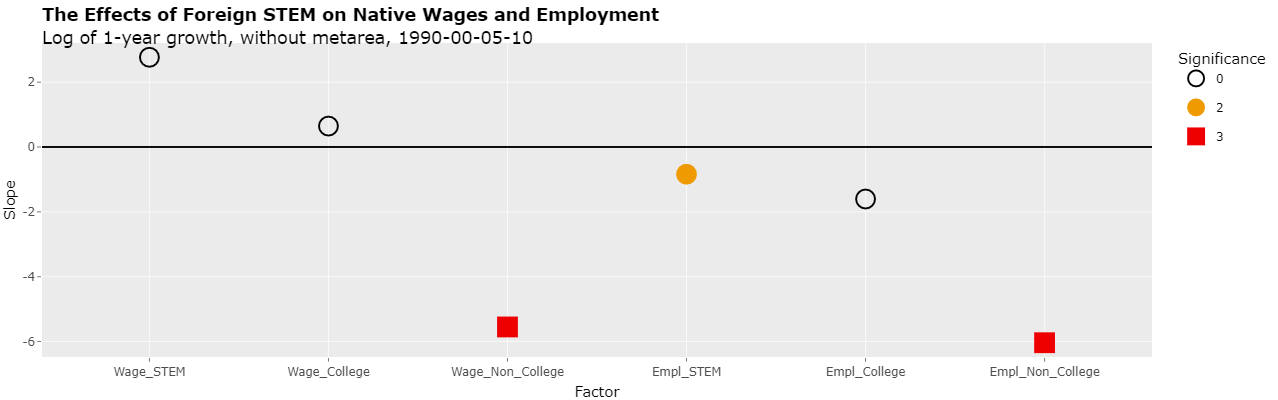
As can be seen, the slopes of the regressions have the same general relationship as before the logs of the annualized growth rates were applied. The slopes of the last 4 regressions are now negative and 3 of them are with some level of significance.
It should be noted that this analysis assumes that the original data in PSS_Data.dta, which came from the study, is correct. There is some analysis of that data at this link.
Comparing Only Time Spans of the Same Length
Another way to show the effect of the study doing a regression using time spans of different lengths is to follow the study's methods but only include time spans of the same length. In this way, there's no need to annualize growth rates since all time spans are the same length. Time spans of 10 years can be used by including 1990-2000 and 2000-2010. Selecting "1990-00-10" in the "Time spans" select list (with "Timespan growth", "Use metareas", and "Cluster(metareas) selected) displays the following plot:
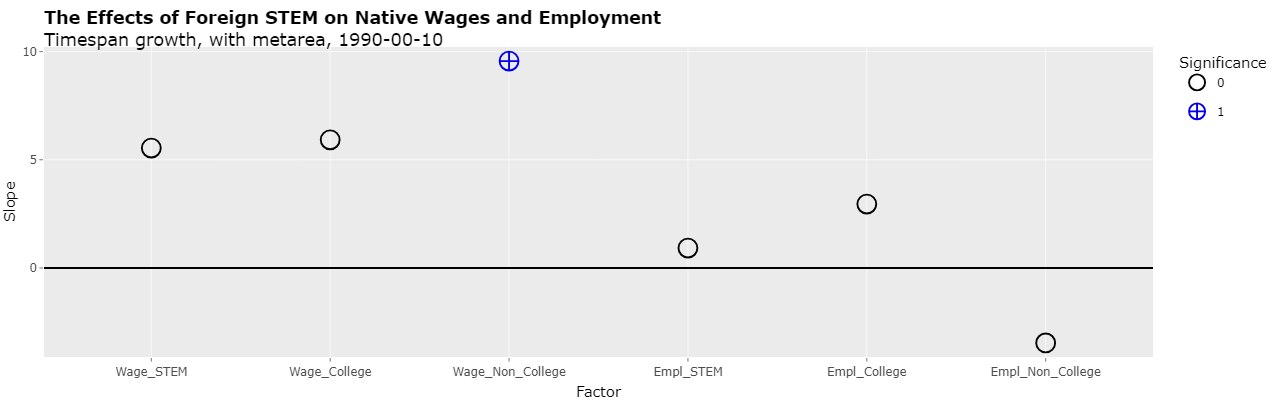
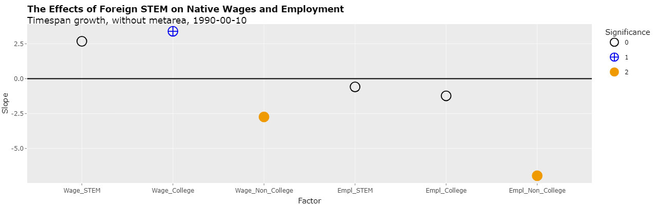
As can be seen, there is now only one p-value with significance and it's significance is fairly low (at the 10% level). However, now using metareas as an indicator variable essentially creates a coefficient for every 2 data points. Removing the use of metareas now results in 3 significant p-values, the most significant two of which have negative slopes as shown below:
In any event, time spans of 5 years can be used by including 2000-2005 and 2005-2010. Selecting "2000-05-10" in the "Time spans" select list (with "Timespan growth", "Use metareas", and "Cluster(metareas) selected) displays the following plot:
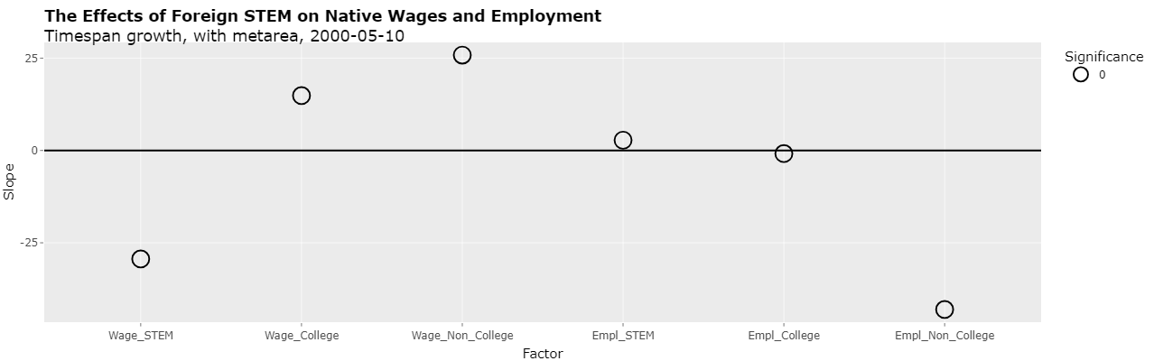
As can be seen, none of the p-values are significant. Hence, this is further evidence that the significant p-values in the first line of Table 5 depended on a regression which incorrectly mixed growth rates from time spans of different lengths.
Recent References to the Study
The study continues to be referenced. For example, Giovanni Peri referenced the paper in an Econofact podcast on January 31, 2022. At about 5:29 in the podcast, Peri said the following as can be seen in the transcript:
In a paper that I published in 2016 with Chad Sparber and Kevin Shih, we analyzed the change of the H1B visa program, which has been the visa program bringing in the US as main channel of entry, the largest part of highly educated immigrant, working in science and technology. So in that study, looking at US location[s] where the number of foreign scientists and engineer increased the most from 1990 to 2010, as a consequence of this H-1B program, we found that those locations where also where productivity grew the most. Not only. Those were the location where wages and employment of US college educated grew faster. In fact, we calculated that about half of the productivity growth of the average US location in that period could be attributed to the growth of productivity driven by foreign born STEM workers.