1. The Claim that Each Additional 100 H-1B Workers Create an Additional 183 Native Jobs
A study titled "Immigration and American Jobs", written by economist Madeline Zavodny, was released by the American Enterprise Institute and the Partnership For A New American Economy in December of 2011. On page 4 of this study, the second main finding states that "[a]dding 100 H-1B workers results in an additional 183 jobs among US natives." This is expanded upon on page 11 which states:
The estimates show that a 10 percent increase in H-1B workers, relative to total employment, is associated with a 0.11 percent increase in the native employment rate. During the sample period of 2001–2010, this translates into each additional 100 approved H-1B workers being associated with an additional 183 jobs among US natives.
The data used to reach this finding is explained on page 16 as follows:
The Department of Labor publishes data on applications for temporary foreign workers through the H-1B, H-2A, and H-2B programs. Those data are used here for the years they are available: 2001–2010 for the H-1B program, 2006–2010 for the H-2A program, and 2000–2010 for the H-2B program.[29] The measure of temporary foreign workers used here is the number of approved foreign workers in a given state and year. These counts of approved workers proxy for the ultimate number of new temporary foreign workers in each state, since data on actual temporary foreign worker inflows by geographic area are not available.[30]
Hence, the study is using the number of approved workers as proxy for the ultimate number of actual workers. In addition, this explanation refers to footnote 29 on page 23 which start as follows:
The data are from Foreign Labor Certification Data Center, www.flcdatacenter.com (accessed November 12, 2011), and are for fiscal years. The public-use H-1B data for 2007 contain erroneous codes for the work state, so the analysis here does not include that year.
For that reason, 2007 is likewise excluded for this replication. The following table shows the study's key H-1B data by year.
          TABLE 1: H1B AND NATIVES: NUMBER EMPLOYED AND LEVELS, BY YEAR

year    emp_h1b   emp_native    emp_total   pop_native  h1b_level  nat_level  ln_h1b_level  ln_nat_level
----  ---------  -----------  -----------   ----------  ---------  ---------  ------------  ------------
2001  1,432,702  102,771,951  119,489,933  155,359,951  1.1990148   66.15086     0.1815002      4.191938
2002    644,581  101,993,592  118,798,501  157,039,250  0.5425834   64.94783    -0.6114134      4.173584
2003    512,697  101,737,445  119,047,895  159,092,173  0.4306645   63.94874    -0.8424260      4.158082
2004    627,326  102,441,401  120,166,278  160,589,716  0.5220483   63.79076    -0.6499952      4.155608
2005    682,013  104,114,426  122,535,961  162,271,513  0.5565819   64.16063    -0.5859409      4.161390
2006    628,951  105,253,440  124,517,864  163,469,261  0.5051090   64.38730    -0.6829809      4.164916
2008    658,604  105,480,298  124,964,666  165,699,739  0.5270322   63.65749    -0.6404937      4.153517
2009    517,196  101,483,644  120,106,722  167,119,661  0.4306137   60.72514    -0.8425439      4.106358
2010    498,434  100,668,333  119,534,797  167,863,135  0.4169782   59.97048    -0.8747214      4.093852
Columns 2 and 3 are the number of employed h-1b and natives and columns 4 and 5 are the total employed and total native population. Columns 6 is the "h-1b level" and equals 100 times the employed h-1b (column 2) divided by the total employed (column 4). Column 7 is the "native level" and equals 100 times the employed natives (column 3) divided by the total native population (column 5). Columns 8 and 9 are just the logs of the levels in columns 6 and 7, respectively. These are the key numbers in the regressions.
As can be seen, employed h-1b (column 2) for 2001 is more than double its value for 2002 and later years. I looked at this several years ago and wrote the following at this link:
It should be noted that many applications did request just under 1,000 worker positions. I would assume that requests of 999 and slightly less often served as placeholders when large numbers of positions were desired but the exact number was unknown. The relatively large number of such requests in 2001 caused the total number of work positions to be over 1.4 million.
Because of this, the number of workers approved in 2001 may be far greater than the final actual number. In fact, the second table at this link shows that only 331,206 H-1B petitions were approved in 2001. Hence, the Labor Condition Applications (LCAs) may be a very poor proxy for the actual H-1B worker inflow per state since their is no guarantee that states will have similar ratios of certified to actual workers. Finally, it should be noted that this is only a proxy (likely a poor one) for the new H-1B workers. It reveals nothing about the cumulative number of such workers.
In any case, following table shows the results of regressions on the study's H-1B data:
[1] "TABLE 2: RESULTS OF REGRESSIONS ON STUDY'S H-1B DATA                          "
[1] "                                                                              "
[1] "                           JOBS    CORREL                                     "
[1] " N  INTERCEPT    SLOPE   CREATED    COEF   DESCRIPTION                        "
[1] "--  ---------  --------  -------  -------  -----------------------------------"
[1] "2001-2010, ALL DATA"
[1] " 1)   -0.3193    0.0219    326.4   0.2989  ln_nat_level ~ ln_imm_level"
[1] " 2)   -0.3227    0.0170    253.6   0.2989  ln_nat_level ~ ln_imm_level + fyear"
[1] " 3)   -0.4718   -0.0008    -11.5   0.2989  ln_nat_level ~ ln_imm_level + fyear + floc"
[1] " 4)   -0.3956    0.0110    182.5   0.2989  ln_nat_level ~ ln_imm_level + fyear + floc, weights=weight"
[1] "USING STUDY'S FORMULA"
[1] " 5)   -0.3956    0.0115    171.6   0.2989  2001-2010, study's data with corrected job count"
[1] " 6)   -0.4265    0.0081    140.3   0.2439  2002-2010, skip bad data for 2001"
[1] " 7)   -0.4912   -0.0023    -37.6   0.2177  2002-2008, skip worse years of job loss"
[1] " 8)   -0.5230   -0.0064   -108.3   0.2142  2003-2006, skip all years of job loss"
[1] " 9)   -0.5716   -0.0132   -223.4   0.2450  2003-2005, longest span of growing h1b level"
Regressions 1 to 4 show the results of the regression after adding each additional variable. The variable fyear is a dummy variable for year, floc is a dummy variable for the state, and weight is a weight used by the study. The weight is based on the native population of each state in each year. Regression 4 is the one on which the study's 183 number is based. However, it appears that Zavodny used the total number of H-1B workers from 2001 to 2010 but the total number of native workers from 2000 to 2010 for the calculation. She also used 0.011 for the slope instead of the exact slope, shown to be about 0.0115 above. After I corrected the calculation to use 2001 to 2010 for both H-1B and native workers and used the more precise measurement of slope, I got 171.6 for the calculated number of jobs created. Using the mismatched time spans and a slope of 0.11 like the study, I came up with 182.5, replicating the study. Similarly, the calculated slope of 0.0115 replicates the study's finding of 0.011 for the slope.
Regressions 5 to 9 show the results using the study's formula for different spans of years. The reason for looking at different spans of years is that the study claims to be looking at jobs being created due to an increase in the level of H-1B workers. It therefore makes sense to look at spans of years when the level of H-1B workers is rising. Certainly, one could claim that decreasing the level of H-1B workers has a negative effect on the native employment level. However, this occurred most severely after the 2001 tech crash and the 2008 financial crisis. The loss of jobs for both H-1B and natives was likely due to these economic events. In these events, I don't know that anyone would claim that the drop in H-1B workers was an independent event and that caused the drop in native employment. At the very least, there was likely a very different dynamic at work during these periods and they should be measured separately. In any event, the table shows that, when focusing on those years for which there were job gains for H-1B workers, those gains, on average, were correlated with drops in native employment, at least when using the study's own methodology.
The following table shows the slopes obtained for all spans of two or more years using the same formula that the study used to obtain the 183 figure. The figures in red are negative and indicate a negative correlation between H-1B and native employment level over the given time spans when using the study's methodology.
[1] "TABLE 3: SLOPE BETWEEN GIVEN YEARS (using same regression as was used to obtain 183 job finding)"
[1] "----  ------  ------  ------  ------  ------  ------  ------  ------  ----"
[1] "year    2003    2004    2005    2006    2007^   2008    2009    2010  year"
[1] "----  ------  ------  ------  ------  ------  ------  ------  ------  ----"
[1] "2001  0.0071  0.0048  0.0014  0.0049    NA    0.0043  0.0104  0.0115  2001"
[1] "2002         -0.0030 -0.0095 -0.0035    NA   -0.0023  0.0069  0.0081  2002"
[1] "2003                 -0.0132 -0.0064    NA   -0.0041  0.0061  0.0070  2003"
[1] "2004                         -0.0104    NA   -0.0047  0.0084  0.0079  2004"
[1] "2005                                    NA   -0.0018  0.0097  0.0066  2005"
[1] "2006                                          0.0010  0.0073  0.0009  2006"
[1] "2007                                                 -0.0192 -0.0152  2007"
[1] "2008                                                         -0.0152  2008"
The following table shows the corresponding jobs gained or lost using the same formula that the study used to obtain the 183 figure. As previously mentioned, however, it appears that the study incorrectly uses 2000-2010 for the native employment instead of 2001-2010 as with H-1B employment. Also, the study appears to have truncated the above slopes to 3 decimal places as shown in Table 4 of the study. As before, the figures in red are negative and indicate a drop in native employment levels when using the study's methodology.
[1] "TABLE 4: JOBS GAINED/LOST BETWEEN GIVEN YEARS (with incorrect native employment in 1st row and truncation errors in all rows)"
[1] "----  ------  ------  ------  ------  ------  ------  ------  ------  ----"
[1] "year    2003    2004    2005    2006    2007^   2008    2009    2010  year"
[1] "----  ------  ------  ------  ------  ------  ------  ------  ------  ----"
[1] "2001   110.7    63.7    15.8    63.7    NA      63.8   162.8   182.5# 2001"
[1] "2001    82.8    50.8    13.2    54.6    NA      55.8   144.7   164.2* 2001"
[1] "2002           -68.6  -166.3   -66.6    NA     -49.6   101.5   138.1  2002"
[1] "2003                  -236.9  -118.1    NA     -83.5   102.7   104.9  2003"
[1] "2004                          -177.0    NA     -80.3   133.3   120.0  2004"
[1] "2005                                    NA     -32.0   150.7   103.9  2005"
[1] "2006                                             0.0   121.1     0.0  2006"
[1] "2007                                                  -352.0  -294.0  2007"
[1] "2008                                                          -294.0  2008"

# value is 182.5 if 2000-2010 is incorrectly used for total native employment and the slope is truncated.
* value is 164.2 if 2001-2010 is correctly used for total native employment but the slope is truncated.
^ the study excludes 2007 stating "[t]he public-use H-1B data for 2007 contain erroneous codes for the work state,
  so the analysis here does not include that year."
The following table shows the corresponding jobs gained or lost using the same formula that the study used to obtain the 183 figure but with no truncation or other errors. As before, the figures in red are negative and indicate a drop in native employment levels when using the study's methodology.
[1] "TABLE 5: NATIVE JOBS GAINED/LOST PER EACH 100 NEW H-1B WORKERS BETWEEN GIVEN YEARS (using the study's methodology with no errors)"
[1] "----  ------  ------  ------  ------  ------  ------  ------  ------  ----"
[1] "year    2003    2004    2005    2006    2007^   2008    2009    2010  year"
[1] "----  ------  ------  ------  ------  ------  ------  ------  ------  ----"
[1] "2001    83.5    61.2    18.9    66.2    NA      59.4   150.6   171.6* 2001"
[1] "2002           -51.5  -157.3   -59.0    NA     -37.6   115.9   140.3  2002"
[1] "2003                  -223.4  -108.3    NA     -68.6   104.2   122.2  2003"
[1] "2004                          -168.1    NA     -76.2   139.1   135.7  2004"
[1] "2005                                    NA     -29.4   162.7   114.9  2005"
[1] "2006                                            15.6   126.0    17.0  2006"
[1] "2007                                                  -338.8  -278.6  2007"
[1] "2008                                                          -278.6  2008"

* value is 171.6 if 2001-2010 is correctly used for total native employment and the slope is not truncated.
^ the study excludes 2007 stating "[t]he public-use H-1B data for 2007 contain erroneous codes for the work state,
  so the analysis here does not include that year."
The p-value is the standard method that statisticians use to measure the "significance" of their analyses. Wikipedia defines it as follows:
In statistics, the p-value is a function of the observed sample results (a statistic) that is used for testing a statistical hypothesis. Before performing the test a threshold value is chosen, called the significance level of the test, traditionally 5% or 1% [1] and denoted as alpha. If the p-value is equal or smaller than the significance level (alpha), it suggests that the observed data are inconsistent with the assumption that the null hypothesis is true, and thus that hypothesis must be rejected and the alternative hypothesis is accepted as true. When the p-value is calculated correctly, such a test is guaranteed to control the Type I error rate to be no greater than alpha.
Table 2 of the study showed that the regression on which the 2.6 job claim is made had a p-value such that 0.05 < p-value < 0.1. Following is one rough description of how to interpret a p-value:
0.10  < P          No evidence against the null hypothesis. The data appear to be consistent with the null hypothesis.
0.05  < P < 0.10   Weak evidence against the null hypothesis in favor of the alternative.
0.01  < P < 0.05   Moderate evidence against the null hypothesis in favor of the alternative.
0.001 < P < 0.01   Strong evidence against the null hypothesis in favor of the alternative.
        P < 0.001  Very strong evidence against the null hypothesis in favor of the alternative.
The following table shows the p-values that correspond to the regression slopes in the prior tables:
[1] "TABLE 6: P-VALUE OF REGRESSION SLOPE BETWEEN GIVEN YEARS (using study's methodology)"
[1] "----  ------  ------  ------  ------  ------  ------  ------  ------  ----"
[1] "year    2003    2004    2005    2006    2007    2008    2009    2010  year"
[1] "----  ------  ------  ------  ------  ------  ------  ------  ------  ----"
[1] "2001 0.16534 0.25727 0.71120 0.20737 0.20737 0.27447 0.01220 0.00697  2001"
[1] "2002         0.62295 0.04438 0.43675 0.43675 0.61268 0.14819 0.08908  2002"
[1] "2003                 0.01225 0.21006 0.21006 0.42960 0.26340 0.19463  2003"
[1] "2004                         0.15324 0.15324 0.50799 0.23695 0.23302  2004"
[1] "2005                                 0.19173 0.84628 0.25582 0.38787  2005"
[1] "2006                                         0.96178 0.51965 0.91383  2006"
[1] "2007                                                 0.13328 0.10355  2007"
[1] "2008                                                         0.10355  2008"
In the above table, p-values showing strong evidence (P < 0.01) are colored red, p-values showing moderate evidence (0.01 < P < 0.05) are colored orange, and p-values showing weak evidence (0.05 < P < 0.10) are colored green. Since this includes only 5 points, p-values that show close to weak evidence (0.10 < P < 0.20) are colored blue. In addition, p-values corresponding to negative slopes are in bold lettering.
As can be seen, the smallest p-values are for the spans 2001 to 2010, 2001 to 2009, 2003 to 2005, and 2002 to 2005. Oddly, the first two correspond to a positive slope and the latter two correspond to a negative slope. Even more oddly, the latter two spans are contained within the former two spans. Expanding upon this, it appears that those spans corresponding to a negative slope but having the lowest p-values are those spans which are 7 years or longer and/or which include 2001. However, those spans corresponding to a positive slope but having the lowest p-values tend to be for shorter spans.
One possible explanation for this apparent contradiction is revealed in Table 1. As can be seen, 2001 to 2002 included a massive drop in H-1B approvals with the number dropping by about 55 percent, from 1,432,702 to 644,581. This decline continued to 512,697 in 2003. The number of H-1B approvals then climbed strongly to 682,013 in 2005 and then stabilized somewhat dropping slightly to 658,604 in 2008. They then dropped sharply again, reaching 498,434 in 2010. As explained in the text after Table 1, the number of H-1B approvals may not be that good of a proxy for the number of H-1B workers. Still, if one is attempting to show the positive effects of an increase in H-1B workers, it would seem to make more sense to focus on periods when the number is actually increasing. As mentioned above, the longest period of strong growth in H-1B approvals was from 2003 to 2005. This period is associated with a negative growth and a p-value showing moderate evidence in favor of the alternative hypothesis that a growth in H-1B workers negatively affects the growth in native workers.
In summary, the entire span from 2001 to 2010 gives a low p-value corresponding with a POSITIVE slope but the spans 2002 to 2005, 2005 to 2007, and 2007 to 2010 show relatively low p-values corresponding with NEGATIVE slopes. This apparent contradiction may be due to attempting to fit a single model to periods when H-1B approvals are increasing and periods when H-1B approvals are decreasing. This may be essentially comparing apples and oranges. At the very least, this shows that selecting one time span and not bothering to look at other time spans is a deeply flawed approach.
2. An Initial Look at the Data
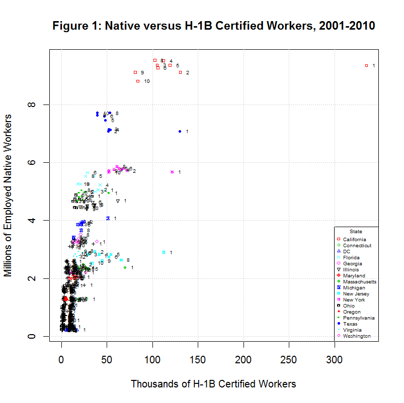
Before looking at the regression that led to the 183 number, it helps to look at the distribution of workers among the states in the following plot:
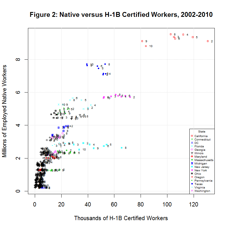
The numbers to the right of each point give the last digit of the year. As can be seen, many of the states have an extremely large number for H-1B workers for 2001. It's unclear what the exact cause of this was. In any event, the following plot omits 2001 so that the other data for other years is more visible:
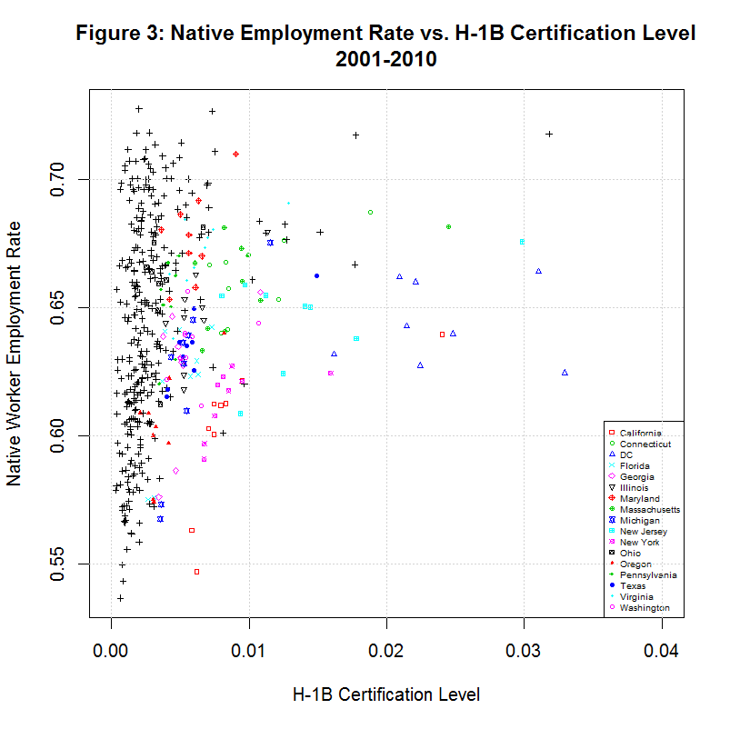
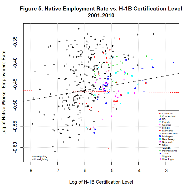
The following plot shows the native employment level verus the H-1B Certification level. Note that the native employment level averages around 65 percent. Hence, this is not the native employment rate but a measure of the native employment divided by the native population.
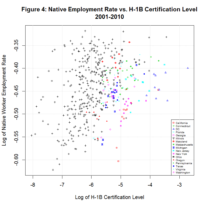
The following two graph show plots of the actual data that is being fit with a regression. The second of the plots show the weighted and unweighted regression of the data. The black line shows the weighted regression that was used by the study to calculate the 183 figure.
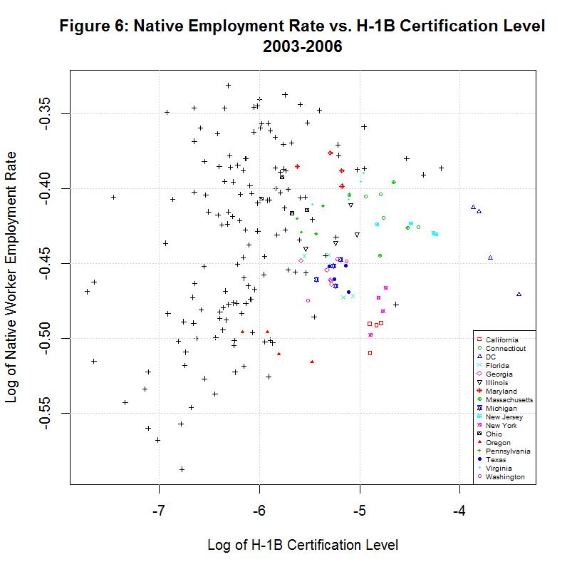
The following two graphs show the same data for 2003 to 2006, a time span when the H-1B level was generally increasing.
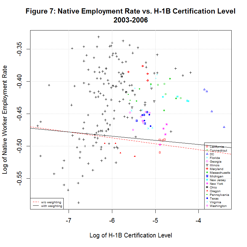
Note that both the weighted and unweighted lines show a negative slope, counter to the study's finding. It should also be noted that the lines do not seem appear to be the best fit of the data. This is caused by the fact that there are dummy variables in addition to the main independent and dependent variable. The cloud-like appearance of the data in these and the prior two graphs suggest that the data is not strongly correlated. However, it is difficult to judge the exact level of correlation since there are more than two variables.
All of the above arguments apply to the 262 number from the study as well. The following table shows the study's key data for this specific class of foreign STEM worker:
TABLE 7: FOREIGN-BORN STEM WORKERS WITH ADVANCED U.S. DEGREE: NUMBER EMPLOYED AND LEVELS, BY YEAR

year   emp_imm   emp_native    emp_total   pop_native  imm_level  nat_level  ln_imm_level  ln_nat_level
----  --------  -----------  -----------  -----------  ---------  ---------  ------------  ------------
2000   148,984  103,082,363  119,167,108  154,182,309  0.1250216   66.85745     -2.079268      4.202563
2001   141,657  102,771,951  119,489,933  155,359,951  0.1185521   66.15086     -2.132403      4.191938
2002   121,521  101,993,592  118,798,501  157,039,250  0.1022919   64.94783     -2.279925      4.173584
2003   151,761  101,737,445  119,047,895  159,092,173  0.1274797   63.94874     -2.059798      4.158082
2004   156,425  102,441,401  120,166,278  160,589,716  0.1301738   63.79076     -2.038885      4.155608
2005   176,080  104,113,290  122,534,825  162,270,376  0.1436980   64.16038     -1.940042      4.161386
2006   175,012  105,253,440  124,517,864  163,469,261  0.1405517   64.38730     -1.962180      4.164916
2007   186,874  105,904,192  125,808,429  164,786,302  0.1485389   64.26759     -1.906909      4.163056
2008   185,667  105,480,298  124,964,666  165,699,739  0.1485759   63.65749     -1.906659      4.153517
2009   203,877  101,483,644  120,106,722  167,119,661  0.1697470   60.72514     -1.773446      4.106358
2010   177,485  100,668,333  119,534,797  167,863,135  0.1484805   59.97048     -1.907302      4.093852
2011   160,208  101,328,629  120,445,461  168,384,994  0.1330134   60.17676     -2.017305      4.097286
2012   199,521  102,432,985  122,263,732  168,723,889  0.1631893   60.71042     -1.812844      4.106115
2013   207,956  103,388,318  123,574,162  169,356,101  0.1682847   61.04788     -1.782098      4.111659
The following table shows the results of regressions on the study's data:
[1] "TABLE 8: RESULTS OF REGRESSIONS REGARDING STUDY'S 262 JOB FINDING             "
[1] "                                                                              "
[1] "                           JOBS    CORREL                                     "
[1] " N  INTERCEPT    SLOPE   CREATED    COEF   DESCRIPTION                        "
[1] "--  ---------  --------  -------  -------  -----------------------------------"
[1] "2000-2007, ALL DATA"
[1] " 1)   -0.4284   -0.0073   -481.1  -0.0640  ln_nat_level ~ ln_imm_level + ln_imm_level2"
[1] " 2)   -0.3998   -0.0054   -356.0  -0.0640  ln_nat_level ~ ln_imm_level + ln_imm_level2 + fyear"
[1] " 3)   -0.4316    0.0021    137.3  -0.0640  ln_nat_level ~ ln_imm_level + ln_imm_level2 + fyear + floc"
[1] " 4)   -0.4167    0.0040    263.0  -0.0640  ln_nat_level ~ ln_imm_level + ln_imm_level2 + fyear + floc, weights=weight"
[1] "USING STUDY'S FORMULA"
[1] " 5)   -0.4167    0.0045    293.4  -0.0640  2000-2007, study's data with corrected job count"
[1] " 6)   -0.5193   -0.0005    -32.2  -0.0299  2002-2005, during first span of increasing immigrant level"
[1] " 7)   -0.4772   -0.0036   -198.2  -0.1662  2006-2009, during second  span of increasing immigrant level"
[1] " 8)   -0.4862   -0.0020   -121.1  -0.1111  2002-2009, during increasing immigrant level (except 2005-06)"
Regressions 1 to 4 show the results of the regression after adding each additional variable. The variable fyear is a dummy variable for year, floc is a dummy variable for the state, and weight is a weight used by the study. The weight is based on the native population of each state in each year. Regression 4 is the one on which the study's 262 number is based. The calculated value was actually just under 263 and the study appears to truncate it to 262. This value, in turn, appears to be based on a truncated value for the slope of 0.004. When using the exact slope, shown to be about 0.0045 above, I came up with a calculated job gain of 293. However, regressions 6 through 9 show that when looking at periods of growth in the level of the foreign stem worker being studied, the level of native workers dropped according to the study's formula.
The following tables show the slopes obtained for all time spans of 3 or more years between 2000 and 2013 and the corresponding native gained or lost:
TABLE 9: SLOPE BETWEEN GIVEN YEARS (using same regression as was used to obtain 262 job finding)
---- ------- ------- ------- ------- ------- ------- ------- ------- ------- ------- -------  ----
Year    2003    2004    2005    2006    2007    2008    2009    2010    2011    2012    2013  Year
---- ------- ------- ------- ------- ------- ------- ------- ------- ------- ------- -------  ----
2000  0.0034  0.0043  0.0040  0.0038  0.0045  0.0025  0.0015  0.0018  0.0025  0.0036  0.0038  2000
2001 .......  0.0044  0.0038  0.0036  0.0043  0.0018  0.0008  0.0012  0.0019  0.0031  0.0033  2001
2002 ....... ....... -0.0005 -0.0009  0.0005 -0.0018 -0.0020 -0.0011 -0.0002  0.0012  0.0017  2002
2003 ....... ....... ....... -0.0006  0.0001 -0.0027 -0.0027 -0.0019 -0.0008  0.0009  0.0014  2003
2004 ....... ....... ....... ....... -0.0012 -0.0035 -0.0030 -0.0022 -0.0010  0.0009  0.0013  2004
2005 ....... ....... ....... ....... ....... -0.0058 -0.0044 -0.0034 -0.0020  0.0001  0.0007  2005
2006 ....... ....... ....... ....... ....... ....... -0.0036 -0.0030 -0.0020  0.0002  0.0009  2006
2007 ....... ....... ....... ....... ....... ....... .......  0.0002  0.0006  0.0025  0.0024  2007
2008 ....... ....... ....... ....... ....... ....... ....... ....... -0.0005  0.0015  0.0013  2008
2009 ....... ....... ....... ....... ....... ....... ....... ....... .......  0.0019  0.0016  2009
2010 ....... ....... ....... ....... ....... ....... ....... ....... ....... .......  0.0026  2010

TABLE 10: JOBS GAINED/LOST BETWEEN GIVEN YEARS (using same regression as was used to obtain 262 job finding but with truncation errors)
---- ------- ------- ------- ------- ------- ------- ------- ------- ------- ------- -------  ----
Year    2003    2004    2005    2006    2007    2008    2009    2010    2011    2012    2013  Year
---- ------- ------- ------- ------- ------- ------- ------- ------- ------- ------- -------  ----
2000  217.89  284.32  274.93  269.32  262.99  129.20  125.53  124.35  124.53  245.06  241.05  2000
2001 .......  286.29  274.57  268.11  261.14  128.14   62.13   61.55  123.40  182.06  179.01  2001
2002 ....... .......    0.00  -66.03    0.00 -126.06 -122.07  -60.54    0.00   59.80  117.60  2002
2003 ....... ....... .......  -62.73    0.00 -181.70 -176.36 -117.05  -59.01   58.14   57.26  2003
2004 ....... ....... ....... .......  -60.16 -178.35 -172.89 -115.00  -58.15   57.31   56.45  2004
2005 ....... ....... ....... ....... ....... -348.87 -225.22 -169.11 -114.48    0.00   55.60  2005
2006 ....... ....... ....... ....... ....... ....... -222.57 -167.55 -113.87    0.00   55.19  2006
2007 ....... ....... ....... ....... ....... ....... .......    0.00   56.32  110.86  109.06  2007
2008 ....... ....... ....... ....... ....... ....... ....... .......    0.00   55.18   54.18  2008
2009 ....... ....... ....... ....... ....... ....... ....... ....... .......  109.54  107.33  2009
2010 ....... ....... ....... ....... ....... ....... ....... ....... ....... .......  164.18  2010

TABLE 11: NATIVE JOBS GAINED/LOST PER EACH 100 STEM WORKERS WITH ADVANCED US DEGREES BETWEEN GIVEN YEARS (using study's methodology with no errors)
---- ------- ------- ------- ------- ------- ------- ------- ------- ------- ------- -------  ----
Year    2003    2004    2005    2006    2007    2008    2009    2010    2011    2012    2013  Year
---- ------- ------- ------- ------- ------- ------- ------- ------- ------- ------- -------  ----
2000  245.51  306.94  274.79  257.13  293.44  158.33   96.35  112.38  154.98  221.82  225.99  2000
2001 .......  317.81  262.67  242.41  280.19  114.42   46.88   73.19  117.79  188.00  194.49  2001
2002 ....... .......  -32.21  -59.12   30.37 -110.55 -121.07  -65.43  -12.20   74.36   98.75  2002
2003 ....... ....... .......  -39.24    3.18 -162.83 -161.62 -108.66  -47.03   50.47   78.46  2003
2004 ....... ....... ....... .......  -70.56 -206.88 -175.46 -125.54  -57.93   52.45   72.69  2004
2005 ....... ....... ....... ....... ....... -338.56 -249.66 -189.44 -114.91    4.97   41.33  2005
2006 ....... ....... ....... ....... ....... ....... -198.23 -168.66 -115.45    8.89   50.58  2006
2007 ....... ....... ....... ....... ....... ....... .......   13.27   33.91  136.92  132.92  2007
2008 ....... ....... ....... ....... ....... ....... ....... .......  -27.36   82.76   73.07  2008
2009 ....... ....... ....... ....... ....... ....... ....... ....... .......  101.55   83.93  2009
2010 ....... ....... ....... ....... ....... ....... ....... ....... ....... .......  142.78  2010

# value is 262.99 if the slope is truncated.
* value is 293.44 if the slope is not truncated.
As with the H-1B data, the table above shows that when one looks at a time span for which the foreign worker being studied is increasing, a loss of native jobs is indicated. For example, 2002 to 2009 shows an steady increase in such workers and their share of the employment pool was generally increasing. The table, however, shows a negative slope of -0.0020 during this period, indicating a loss of native jobs.
The following table shows the p-values that correspond to the slopes in the prior tables:
TABLE 12: P-VALUE OF REGRESSION SLOPE BETWEEN GIVEN YEARS (using study's methodology)
---- ------- ------- ------- ------- ------- ------- ------- ------- ------- ------- -------  ----
Year    2003    2004    2005    2006    2007    2008    2009    2010    2011    2012    2013  Year
---- ------- ------- ------- ------- ------- ------- ------- ------- ------- ------- -------  ----
2000  0.1144  0.0206  0.0307  0.0492  0.0141  0.1631  0.3987  0.3366  0.1956  0.0487  0.0313  2000
2001 .......  0.0425  0.0685  0.0993  0.0330  0.3439  0.6955  0.5476  0.3426  0.1038  0.0688  2001
2002 ....... .......  0.8532  0.7291  0.8360  0.3923  0.3364  0.6081  0.9247  0.5321  0.3633  2002
2003 ....... ....... .......  0.8374  0.9840  0.2334  0.2242  0.4175  0.7269  0.6815  0.4818  2003
2004 ....... ....... ....... .......  0.7145  0.1782  0.2313  0.3912  0.6894  0.6844  0.5275  2004
2005 ....... ....... ....... ....... .......  0.0544  0.1336  0.2368  0.4618  0.9707  0.7241  2005
2006 ....... ....... ....... ....... ....... .......  0.2731  0.3076  0.4641  0.9470  0.6584  2006
2007 ....... ....... ....... ....... ....... ....... .......  0.9417  0.8395  0.3188  0.2376  2007
2008 ....... ....... ....... ....... ....... ....... ....... .......  0.8900  0.5667  0.5138  2008
2009 ....... ....... ....... ....... ....... ....... ....... ....... .......  0.4249  0.4028  2009
2010 ....... ....... ....... ....... ....... ....... ....... ....... ....... .......  0.2039  2010
In the above table, the p-values are colored red if they are less than 0.01 (p < 0.01), orange if they are less than 0.05 (0.01 <= p < 0.05), and green if they are less than 0.1 (0.05 <= p < 0.1). As can be seen, there are no red values of the highest significance but there 8 and 4 of the other two levels, respectively. There is at least one span, 2005 to 2008, that has a p-value less than 0.1 but corresponds to native jobs losses of 348.87 and 338.56 in the prior two tables.
In any event, these numbers show how critical the first and last year of the chosen time span are to the results. This seems to be especially true for certain years such as the tech crash that occurred in 2000-2002. As can be seen in the first table in this section, there was a steep job loss for both foreign and native workers during this period. This underlines an interesting fact. A job increase for both foreign and native workers will result in a regression finding a positive association between the two. However, a steep job loss will result in a regression finding a similar positive association. Since time is not included in the plot, both cases are essentially identical from a mathematical point of view. Of course, the study is not claiming that foreign job LOSSES lead to native job LOSSES. Hence, it makes sense to focus on periods of gains in the jobs of foreign workers. As mentioned above, when looking at periods of growth in the level of the foreign stem worker being studied, the level of native workers generally dropped according to the study's formula.
The following table shows the standard errors that correspond to the slopes in the prior tables:
STANDARD ERROR OF REGRESSION SLOPE BETWEEN GIVEN YEARS (using study's methodology)
---- ------- ------- ------- ------- ------- ------- ------- ------- ------- ------- -------  ----
Year    2003    2004    2005    2006    2007    2008    2009    2010    2011    2012    2013  Year
---- ------- ------- ------- ------- ------- ------- ------- ------- ------- ------- -------  ----
2000  0.0021  0.0018  0.0018  0.0019  0.0018  0.0018  0.0018  0.0019  0.0019  0.0018  0.0017  2000
2001 .......  0.0022  0.0021  0.0022  0.0020  0.0019  0.0019  0.0020  0.0020  0.0019  0.0018  2001
2002 ....... .......  0.0026  0.0026  0.0023  0.0020  0.0021  0.0021  0.0021  0.0020  0.0018  2002
2003 ....... ....... .......  0.0030  0.0026  0.0022  0.0023  0.0023  0.0023  0.0021  0.0019  2003
2004 ....... ....... ....... .......  0.0032  0.0026  0.0025  0.0025  0.0025  0.0022  0.0020  2004
2005 ....... ....... ....... ....... .......  0.0030  0.0029  0.0028  0.0027  0.0024  0.0021  2005
2006 ....... ....... ....... ....... ....... .......  0.0032  0.0029  0.0028  0.0024  0.0021  2006
2007 ....... ....... ....... ....... ....... ....... .......  0.0033  0.0030  0.0025  0.0021  2007
2008 ....... ....... ....... ....... ....... ....... ....... .......  0.0035  0.0026  0.0021  2008
2009 ....... ....... ....... ....... ....... ....... ....... ....... .......  0.0023  0.0019  2009
2010 ....... ....... ....... ....... ....... ....... ....... ....... ....... .......  0.0020  2010
As can be seen, the standard error is between 0.0017 and 0.0022 in the first two rows that correspond to job gains and between 0.0017 and 0.0033 when including all of the spans that correspond to job gains. This compares to 0.0020 and 0.0035 for those spans that correspond to job losses, a relatively small difference.
Source Code for R Programs Used in this Analysis